Presented at SAGEEP 2013, Colorado
For a PDF of this paper click here
Abstract
A new time-domain design implementation for the VTEM helicopter time-domain EM system, known as “Full-waveform” VTEM, addresses the early time issues that have been limiting its shallow mapping capability for near-surface applications.
The Full-waveform design implementation consists of a combination of a) streamed half-cycle recording of transmitter and receiver waveform data, as well as b) continuous system calibration corrections, b) parasitic-noise and transmitter-drift corrections, and d) ideal-waveform-deconvolution corrections that are applied in a separate post-processing step. This leads to an improvement in usable early time data from ~100usec in standard VTEM systems to ~20usec for Full waveform VTEM. This results in a vastly improved near-surface hydrogeologic characterization.
The Full-waveform system and theory were previously described by Legault et al. (2012). This paper presents VTEM case-study examples with emphasis on near-surface applications.
Introduction
Early time or high frequency airborne electromagnetic data (AEM) are desirable for shallow sounding or mapping of resistive areas but this poses difficulties due to a variety of issues, such as system bandwidth, system calibration and parasitic loop capacitance (Macnae and Baron-Hay, 2010).
The Full Waveform (Legault et al., 2012) design implementation of the VTEM (versatile time-domain electromagnetic; Witherly et al., 2004) helicopter system is designed to achieve fully calibrated time-domain EM decays, particularly in early times (<100us), for better near-surface mapping than was previously possible with earlier VTEM helicopter system, while still maintaining its late-channel data quality for deeper penetration. The Full Waveform technology consists of a combination of 1) streamed half-cycle recording of transmitter and receiver waveform data, as well as 2) continuous system calibration corrections, 3) parasitic-noise and transmitter-drift corrections, and 4) ideal-waveform-deconvolution corrections, according to the method described by Macnae and Baron-Hay (2010). The latter three corrections are applied in a separate post-processing step (Legault et al., 2012).
Results of the Full Waveform VTEM surveys have led to improved accuracy of transient data at earlier times than previously achieved – as early as ~20 μs after the current turn-off (versus ~100 μs for standard VTEM) and as late as ~10 ms (channels 4-47). These, in turn, have also led to improvements in the model space that include better definition of the surficial layering and shallow structure, which appear to be in good agreement with known geology, based on case-study results.
Theory and Methodology
Deconvolution of airborne AEM to step response was first proposed by Annan (1986) for the “Prospect” fixed-wing system, which evolved into the Spectrem AEM system, and was later implemented in the Saltmap and Tempest AEM systems (Lane et al, 2000). The Full Waveform VTEM is the first commercial helicopter EM system to adopt waveform deconvolution (Macnae, 2012; Legault et al., 2012).
The sensor calibration procedure uses the measured calibration waveform for corrections of half-cycle waveforms acquired on a survey flight. The half-cycle waveforms of each channel are corrected to obtain the waveforms that would be recorded if the time-domain responses of all the channels, including the reference channel, were from the same Gaussian-like, “ideal” response that is defined by its bandwidth.
A streamed current monitor and streamed receiver data are used for the continuous system response correction, as well as the transmitter drift & parasitic noise corrections, and ideal waveform deconvolution. The deconvolution procedure corrects, in frequency domain, one complete period for linear system imperfections including transmitter current drift through the following operation:

Where R(t) is the desired response (corresponding to R(w) in frequency domain), C is the instantaneous current monitor and C0 the averaged high altitude reference current monitor measurement, B the instantaneous survey data and H0 the averaged high-altitude data respectively. W(w) is an ideal waveform for which the response is desired (Macnae and Baron-Hay, 2010).
The VTEM survey results are initially processed using standard methods, with the system calibration correction and the parasitic-noise/transmitter-drift/ideal-waveform-deconvolution corrections applied in a separate post-processing step using the full-waveform data. The usable early time dBz/dt data following the system response correction and ideal waveform deconvolution typically improves from ~100usec to ~20usec after the end of current turn-off (Legault et al., 2012).
Case Study 1: Spiritwood Valley Aquifer, Manitoba
The Spiritwood Valley was chosen as a test area for the full waveform VTEM system implementation (Legault et al., 2012), based on the availability of previous airborne and ground EM, electrical and seismic, borehole geophysical and well-log data from the study of a shallow freshwater aquifer by the Geological Survey of Canada (Oldenborger et al., 2010, 2011 and 2012). The Spiritwood Valley is a 10-15km wide, 100-150m deep, northwest-southeast trending, buried bedrock valley that extends between Killarney and Cartwright (Figure 1) and extends 500km from Manitoba, across North Dakota and into South Dakota.
The valley lies within a till plain with little topographic relief but has been defined by a series of borehole transects and seismic reflection data collected north of Killarney. The stratigraphy within the valley is variable but includes a basal, shaly sand and gravel, and overlying clay-rich and silty till units. But the sand and gravel is only found in incised valleys, making for a valley-within-valley morphology. The underlying bedrock is conductive, fractured silicious shale. According to borehole resistivity log results, the simplified electrical section consists of three main units: 1) till (40-50 Ω-m), 2) sand & gravel (70-200 Ω-m) and 3) shale (5-50 Ω-m). The high resistivity of the sand and gravel makes it a marker unit for incised valleys that are groundwater targets, as shown in the previous helicopter TEM results in Figure 1b (Oldenborger et al., 2012).
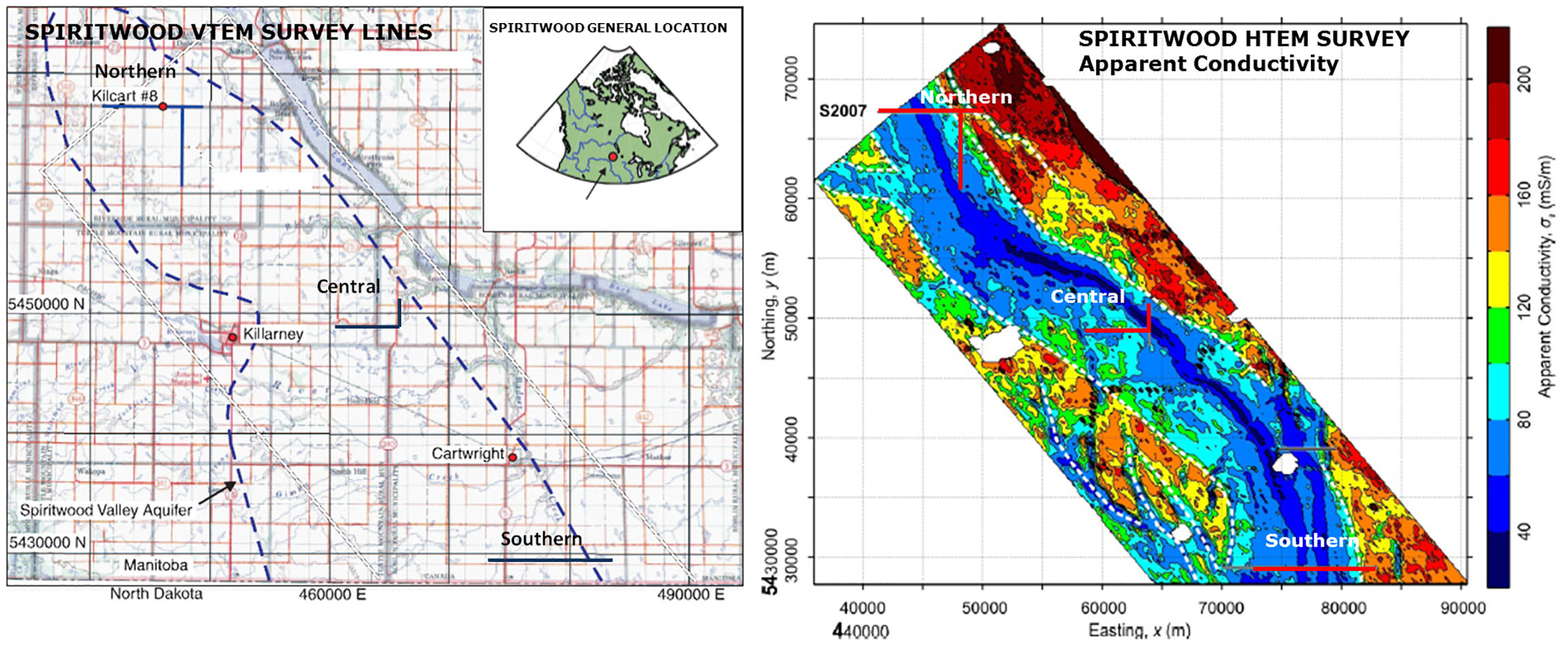
Figure 1. A) Spiritwood Valley location, aquifer outline (blue dash) from geologic mapping and 2011 VTEM test lines (blue solid), and B) Apparent conductivity and aquifer outline (white dash) from 2009 HTEM survey (modified after Oldenborger et al., 2012).
To illustrate the differences and effects of Full Waveform data over regular VTEM, Figure 2 presents Airbeo (Raiche, 1998) 1D layered-earth inversions for both data sets for a representative sounding along the northern line (Figure 1) over the incised valley aquifer where borehole Kilcart #8 is situated. In addition to borehole data, reflection seismic (S2007) and ground electrical tomography (ERI) results (Fig. 3) provide good controls on the layering (Oldenborger et al., 2010). As shown, using the same initial models, the 1D inversion estimates using Full Waveform data (Figure 2a) with better calibrated early times (>18 µs) more closely resemble the known geology – as compared to those from regular VTEM data (Fig. 2b) with later (>96 µs) uncalibrated early-time, whose layering in the upper 30 metres as well as the deeper geoelectrical information (i.e., overestimated resistivity for layer 3) are inaccurate.
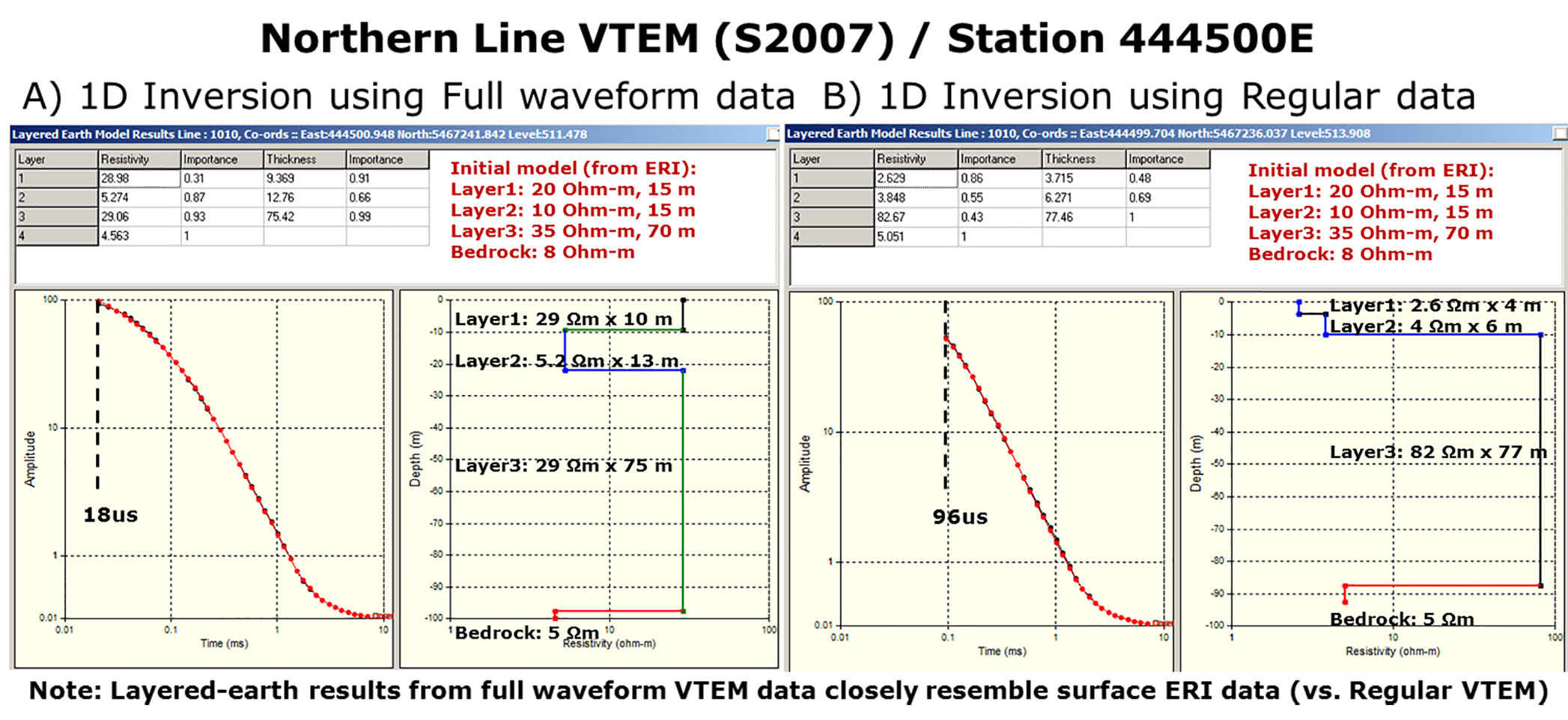
Figure 2. VTEM 1D inversions for northern profile (S2007) from a) Full Waveform and b) Regular data.
Figure 3a shows an example of inverted resistivity models for ERI data acquired at the northern end of the survey area, and compares them to the 3C seismic reflection data for line S2007. The resistivity results show the relatively higher resistivities associated with the deepest part of the valley, suggesting that these sediments are potential aquifer targets. Synthetic modelling of the inversion results shows that the channel anomaly is consistent with erosion of both a supra-bedrock layer (till) and bedrock. The results indicate that ERI provides superior spatial resolution and compare very favourably with the seismic results (Oldenborger et al., 2012).
Figure 3b compares the same 3C seismic and ERI results against 1D spatially-constrained inversion (SCI; Viezzoli et al., 2008) of the Full Waveform VTEM data across the northern survey line. The SCI inversions used an apriori forcing the near surface layers to be resistive, as per the ERI and the known geology. The improvements include better definition of the layering, including the surficial unsaturated till layer (unresolved using standard/non-full waveform VTEM data) and also a more compact resistive anomaly associated with the buried valley aquifer that is in better agreement with previous seismic and resistivity results.
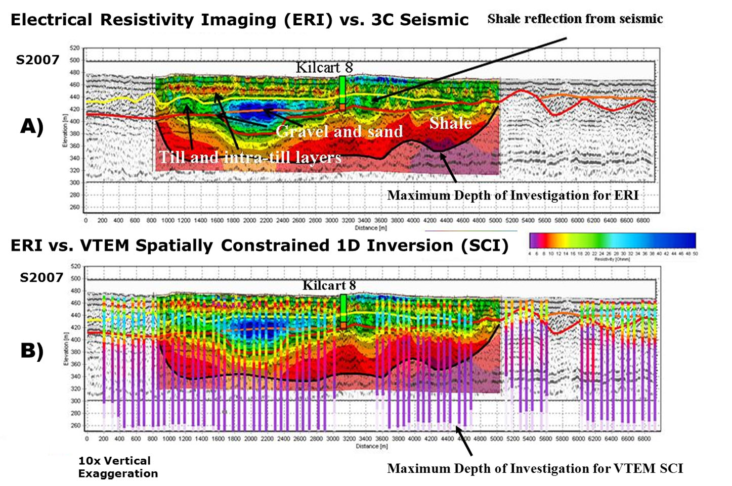
Figure 3. Profile S2007 a) ERI model overlain on interpreted seismic section. Interpreted gravel surface is orange, bedrock surface is red, and gravel-sand layer is yellow. The solid black line indicates the ERI depth of investigation. b) VTEM SCI layered-earth resistivity models overlain on interpreted seismic and ERI sections.
Case Study 2: Timiskaming Kimberlite Field, Northern Ontario
The Timiskaming Kimberlite Field that belongs to Stornoway Diamond Corporation is located 15-40km southwest of Earlton and west of New Liskeard-Haileybury, Ontario (Figure 4a). The field consists of six (6) kimberlite pipe diatremes (95-1, 95-2, (6-1, MR6, KL-01 & KL-22) that are hosted in Proterozoic sediments that are made up of siltstones, argillites, sandstones and conglomerates. The site was chosen as a test area for Full-waveform VTEM because previous HTEM surveys had difficulties detecting these kimberlites, due to high background resistivities and insufficient contrasts.
The 95-2 kimberlite pipe (Figure 4b) is overlain by 30 to 50 metres of overburden. The top 20-30 metres of the pipe contains a cap of weathered tuffusitic kimberlite breccia (WTKB). Below the cap lies the tuffusitic kimberlite breccia (TKB). At depth, a hypabyssal transitional zone has been intersected but not fully explored. 95-2 extends approximately 400 metres in an east-west direction and 80-150 metres from north to south. A geological plan view outline of the extent of 95-2 can be seen in Figure 5a.
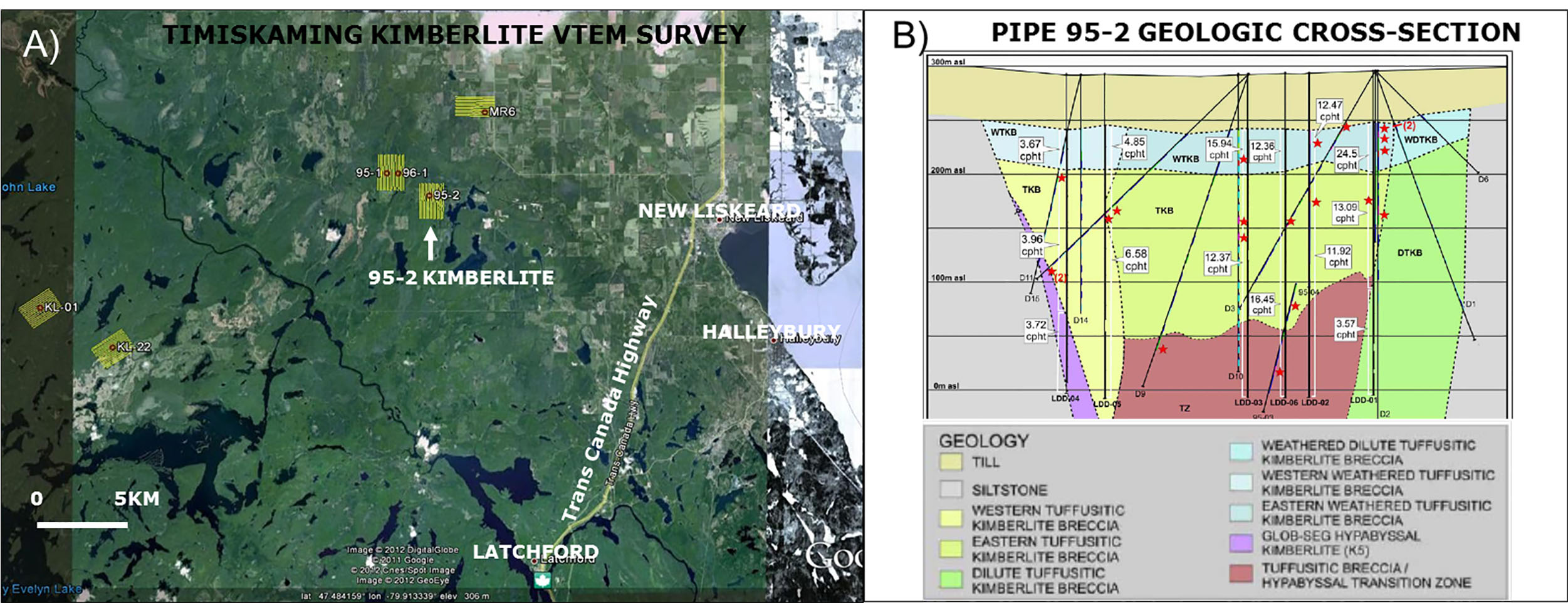
Figure 4. A) Timiskaming Kimberlite VTEM survey locations, showing flight lines (yellow) and kimberlites (red circles); B) Geologic cross-section across 95-2 kimberlite (c/o Stornoway Diamond).
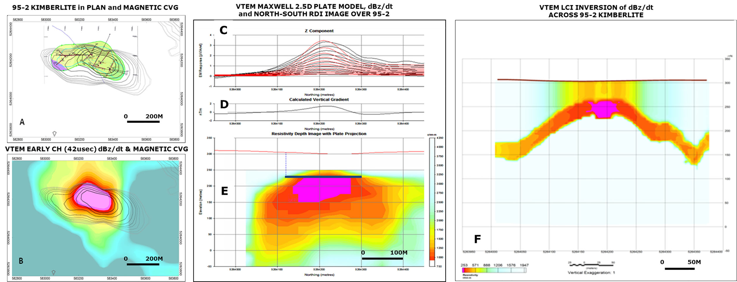
Figure 5. a) Geological Outline of kimberlite pipe 95-2 in plan-view with CVG contours and b) grid of TEM early time gate (ch8 = 39-45 µsec dB/dT) with CVG contours, and VTEM across 95-2: c) dB/dt Z measured ( black) and forward model response (red); d) Calculated vertical gradient of total magnetic intensity; e) Maxwell 2.5D plate model and RDI resistivity depth image, and f) Laterally constrained 1D inversion across north-south Line 1050.
The primary target of EM data modeling is the weathered cap of kimberlite pipes since it is the most conductive and its depth, thickness, conductance and lateral extent can be readily determined. Resistivity-depth images (RDI), seen in Figure 5e, approximate the depth and lateral extent of the kimberlite pipe. However, EM modeling, using the MaxwellTM plate modeling code (EMIT, Midland, WA) yields more accurate results for depth and conductance. The modeled plate for 95-2, shown in blue in Figure 5e, has a 1.1 siemens conductance, is horizontal and lies at a depth of 65 metres. This depth puts the modeled plate precisely in the middle of the weathered kimberlite layer. Based on the RDI, LCI inversion (Auken and Christiansen, 2004) and plate modeling (Figure 5ef), the response is due to the weathered cap of the kimberlite (WTKB). The Timiskaming kimberlites are reflected in EM data with increased response mostly in earliest times, from ~20-120 µsec (Figure 5b). As a result, they would not have been easily discerned with standard/non-full waveform VTEM, with earliest gates at ~100 µsec.
Case Study 3: St. Lawrence Lowlands, Montérégieo Quebec
The Yamaska-Richelieu watershed in the Montérégie East region east of Montreal covers a 9000 km2 area that extends from Sorel to the north and the USA border to the south (Figure 6a). This mainly rural area has a relatively large population density and underground aquifers account for nearly 30% of the >500,000 inhabitants water supply. As part of a larger study since 2009 on the regional groundwater resources, geophysical work has included reflection seismic, regional time-domain electromagnetic (TDEM) soundings, electrical resistivity tomography (ERT) and borehole resistivity logging (Lefebvre et al., 2011). An area at the northern end of the Montérégie East region, situated in the St-Lawrence Lowlands between St-Hyacinthe and Sorel, was selected for Full-waveform VTEM testing along 5 lines that mainly coincide with ground TDEM profiles, totaling 140km (Figure 6a).
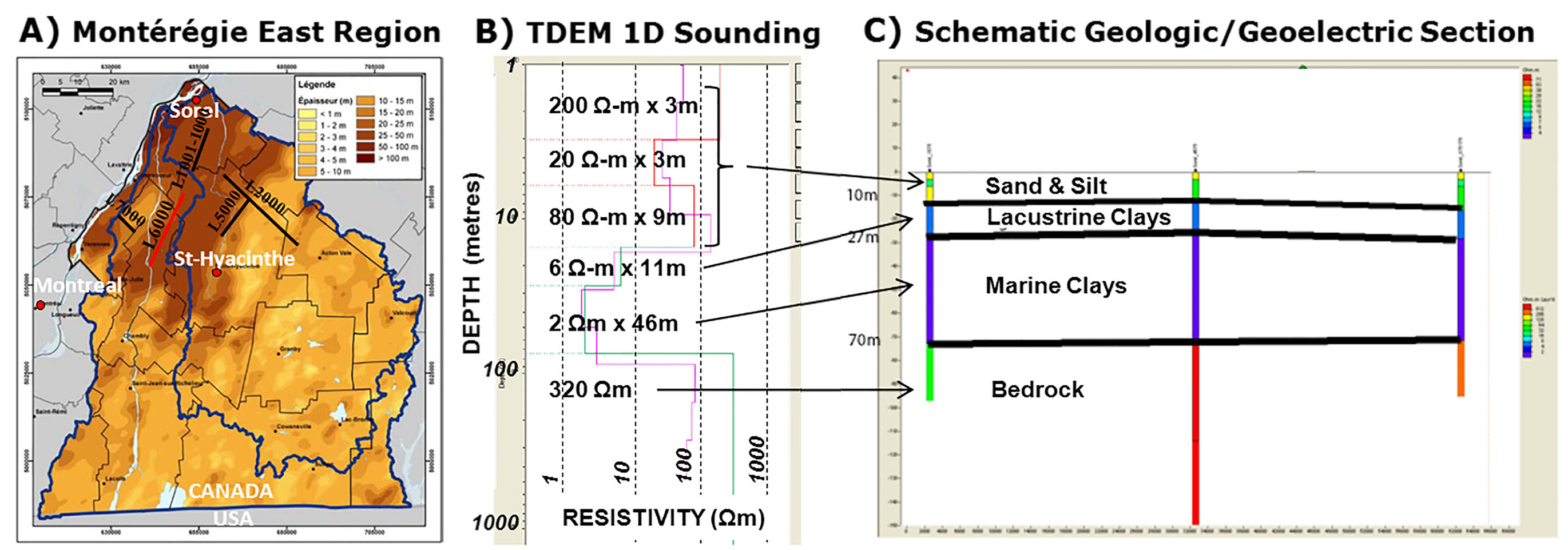
Figure 6: a) Map of Richelieu-Yamaska trans-border aquifer showing sediment thicknesses and VTEM-TDEM survey lines (after Lefebvre et al., 2011); b) TDEM sounding results from Sorel and c) corresponding schematic geologic and geoelectric section (after E. Gloaguen, pers. comm., 2011).
The surficial sediment geology of the St-Lawrence Lowlands typically consist of: 1) glacial tills covering bedrock, at the base, 2) fluvio-glacial sediments, 3) marine silts and clays, and 4) fluvial clays, silts and sands at the surface (Figure 6c). The bedrock is made up of shallow dipping Paleozoic sedimentary rocks, from sandstones at the base, to dolomites, limestones and shales at the top. The thickest clay cover is found from the north of Monteregian Hills to the St. Lawrence River, ranging from 10-70 metres in the VTEM study area (Figure 6a). This same area is also characterized by brackish groundwater (Lefebvre et al., 2011). Time-domain EM sounding data indicate that layer resistivities in the 2-200 ohm-m range match up with the sedimentary layering (Figure 6bc). Saline water infiltration into the basement is also indicated by widely varying basement resistivities (Figure 6c).
Figure 7 presents a pseudo 2D resistivity section from VTEM Full-waveform dBz/dt results along L6000, using an in-house-developed heuristic laterally-constrained inversion (HLCI) that is based on the AirBeo layered earth 1D TEM inversion code of Raiche (1998). 1D LCI inversion (Auken and Christiansen, 2004) results of previous ground TDEM soundings are overlain as thin, vertical resistivity logs. In general the results are very comparable in terms of resistivities and overall thicknesses of the conductive marine clay layer. The VTEM used a different starting model which explains presence of a thin resistive upper layer in the HLCI section, relative to the LCI surficial conductivity. The VTEM data provide results with high lateral resolution (~10m soundings vs. 1km for TDEM) and greater depth of investigation. The VTEM section highlights well-defined paleo-relief features in the basement, and more basement heterogeneity that is consistent with saline water in fractured bedrock. Inconsistencies in the extreme left and right part of the VTEM section are due to powerlines and other man-made culture.
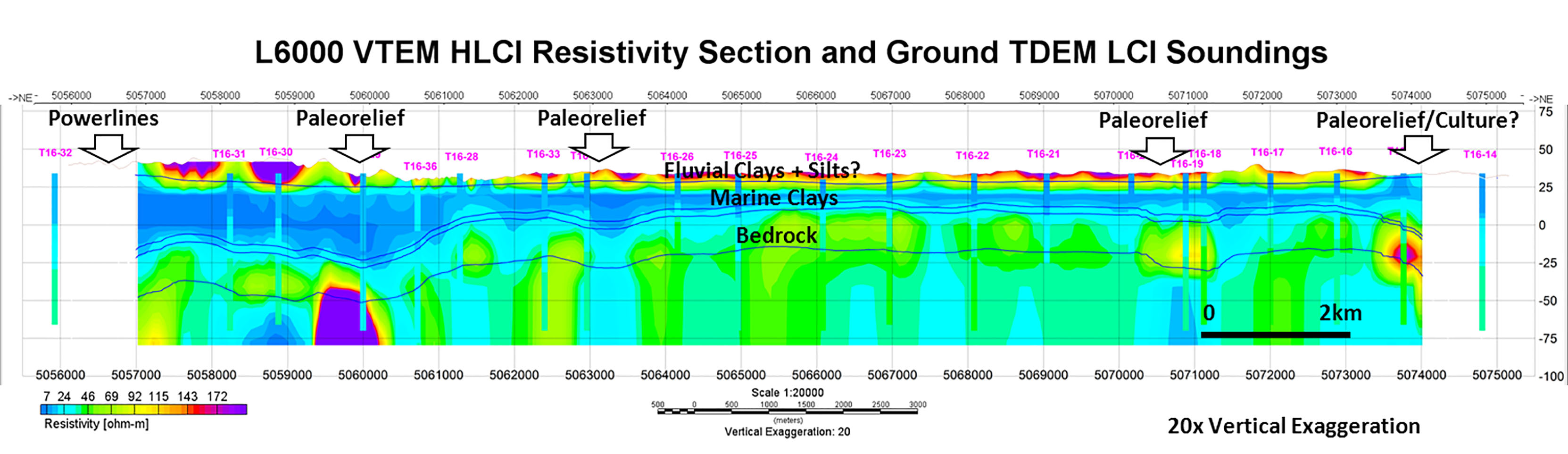
Figure 7: St. Lawrence Lowlands: Pseudo 2D HLCI resistivity section from Full-waveform VTEM along L6000, overlain with LCI resistivity from Ground TDEM soundings, showing layer boundaries (blue lines), major units, sounding sites (red letters) and interpreted basement paleo-relief features.
Case Study 4: Nebraska Sand Hills, Crescent Lakes NWR
The Sand Hills of western Nebraska are the largest dune sea in the western hemisphere and overlie the High Plains aquifer (Smith et al, 2012). Previously, a 2009 helicopter frequency domain EM (HFDEM) survey that was flown in the Crescent Lakes National Wildlife Refuge (NWR) mapped shallow hydrogeologic features of the southwestern part of the Sand Hills that contain a mix of fresh to saline lakes. In 2012, a VTEM helicopter time domain EM survey, using Full-waveform, covered a larger area that overlapped the previous HFDEM and mapped to a greater depth (Smith et al., 2012).
A resistivity depth section obtained from 1D layered earth inversions is shown in Figure 8 for a VTEM line that extends across the Crescent Lakes region and overlaps with a line from the HFDEM survey, shown by the black box. The layered earth resistivity section for the HFDEM survey overlap is presented in Figure 9a, along with the VTEM HLCI section, windowed to the same overlap, in Figure 9b. The shallowest (less than 10 meters) resistivity distribution is best defined by the HFDEM survey, which maps to roughly 40m. However VTEM survey results are generally the same as interpreted from ground TDEM and also map the deeper features to a depth on the order of 300 metres. The dune dam near Crescent Lake is defined by a 45m deep resistive zone (Figure 9) and appears to influence ground-water flow paths and surface-water features. The VTEM results (Figure 8-9b) suggest that, below the resistive sand dunes, the upper part stratigraphy consists of Ogallala silts that overlay more resistive sands. The deepest part of the section consists of electrically conductive Brule shales, which are shallow in the southern end of the section (Figure 8 – left) and deepen to the north (right). This trend is interpreted to influence regional and possibly also the shallower groundwater flow (Smith et al., 2011).
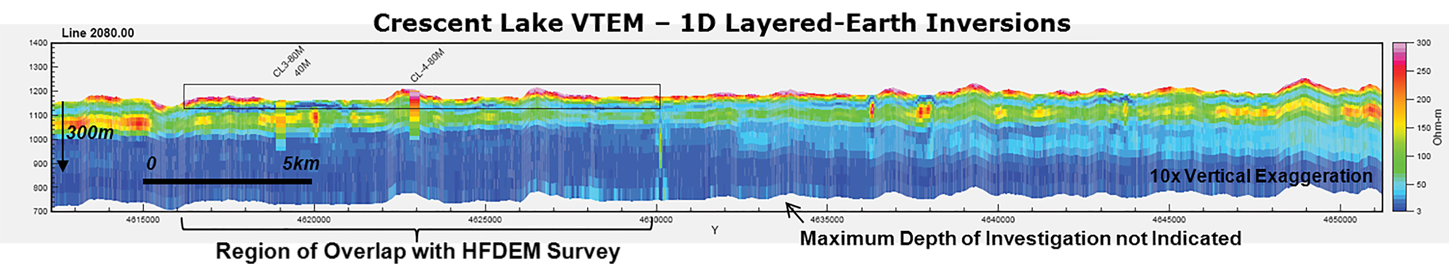
Figure 8: Crescent Lake VTEM pseudo 2D resistivity section from 1D layered-earth inversions (after Smith et al., 2012), showing HFDEM and HTDEM survey overlap.
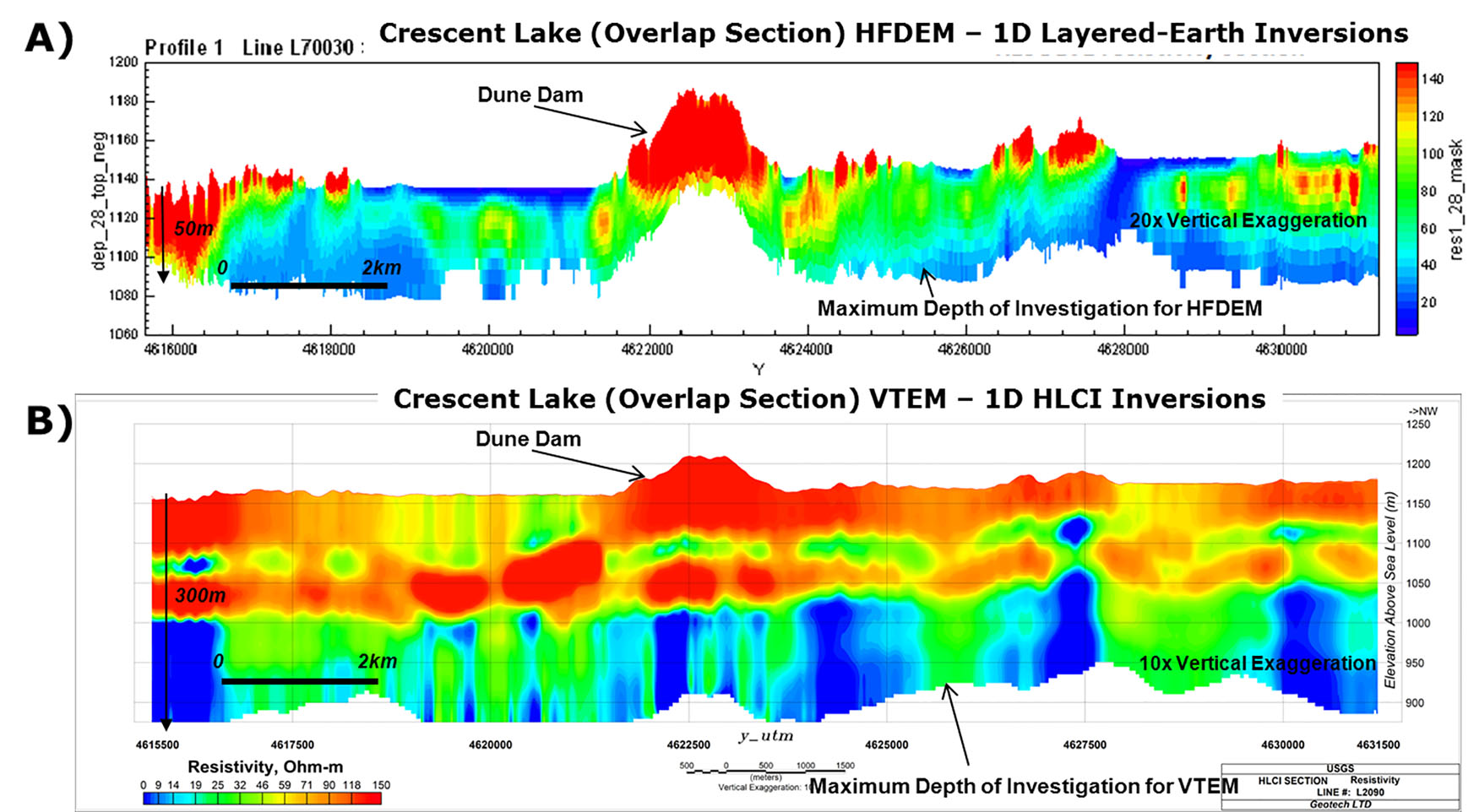
Figure 9: Crescent Lake a) HFDEM resistivity section compared with: b) VTEM HLCI resistivity section across overlap, with the dune dam in the center of the profile.
Case Study 5: Horn River Basin, Northeastern BC
The Horn River Basin in northeastern British Columbia is a significant shale gas play that requires groundwater sources for hydraulic fracturing, which include shallow (<500m) fresh water aquifers in Quaternary sediments or shallow bedrock and deep (>500m) saline aquifers in bedrock (Best et al., 2013). In 2005 Arcis Seismic Solutions of Calgary, Alberta carried out the Ootla 3D seismic survey, whose goal was to map the Horn River shale sequence. In 2010, four lines that contained a shallow seismic feature were also flown with VTEM to determine if any shallow features within the 3D survey area could represent potential shallow paleochannel aquifers. A VTEM system without Full-waveform implementation was used, with off-time dBz/dt data collected in 0.09 to 7.56 ms (channels 14 to 45). time-decay range. The seismic and AEM data along these lines were then jointly interpreted to provide an interpretation of the Quaternary sediments (Best et al., 2013).
Figure 10 presents a depth-migrated seismic section for L1010, in black and white, and the corresponding VTEM LCI inversion overlain in colour. The strong seismic reflector at approximately 540-580m above mean sea level closely follows the bottom of a strong (6-10 ohm-m) conductive layer and a discontinuous weaker reflector tends to line up with the top of the layer. This conductive layer corresponds to the Cretaceous Horn River shale and the more resistive material (> 50 ohm-m) above the shale is the unconsolidated Quaternary sediments. The more resistive values (> 200 ohm-m) within the Quaternary sediments correspond to areas containing coarser material (Best et al., 2013).
Two features can be seen on Line 1010 (Figure 10) on the western and eastern sides that could represent potential paelochannels and are also detected on a parallel line. A third, narrower paleochannel is also interpreted at the far eastern end of L1010. Depressions on the shale surface associated with these indicate areas of potential erosion. The overlying Quaternary sediments have higher resistivity values and the shale appears to be slightly more resistive as well. The seismic reflection pattern within the Quaternary section is more complex in these regions and the shale reflection are more disjointed. The combined seismic and AEM evidence are both consistent with aqueous paleochannels (Best et al. 2013).
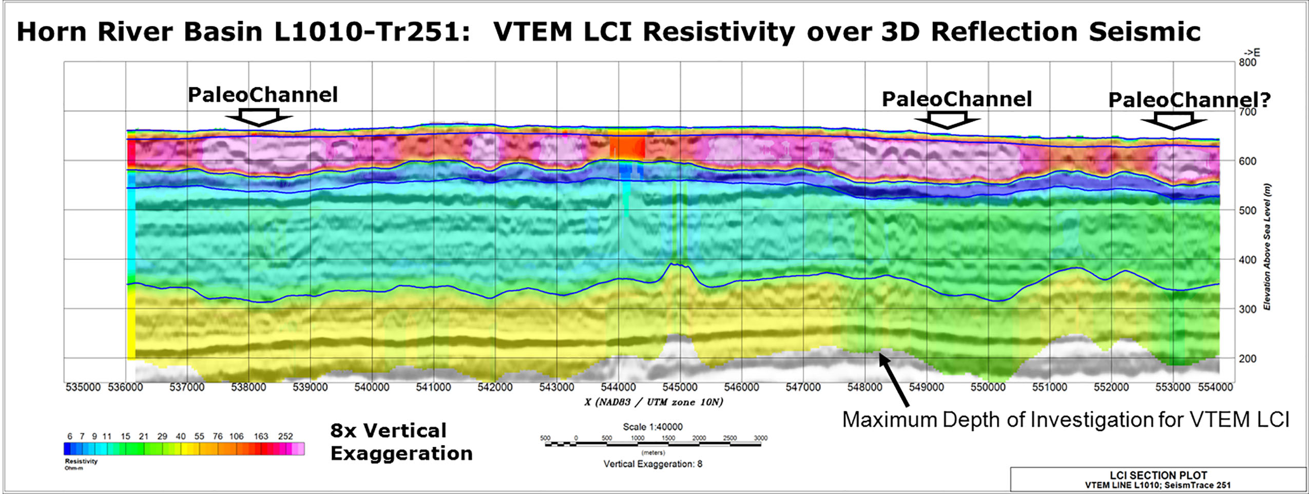
Figure 10: Horn River Basin a) Upper 400 m of the depth migrated 3D seismic section (line 1010) with VTEM LCI inversion overlain in colour, showing potential paleochannels.
Conclusion
Results of a series of Full Waveform VTEM surveys over the aquifers and other near-surface geological case-studies have shown how improvements in quantitative data at earlier times – from approximately 96 µs to as early as 18 µs after the current turn-off and as late as 9.977 ms – can in turn lead to improvements in the model space that include better definition of the surficial layering and shallow structure that are in good agreement with the known geology. Examples include shallow freshwater aquifers in the Spiritwood Valley of southern Manitoba, weathered kimberlite diatremes in the Timiskaming region of northern Ontario, marine clay aquifers in the St. Lawrence Lowlands of eastern Quebec and freshwater aquifers below Sand Hills dunes in western Nebraska. A final example compares standard VTEM to 3D seismic for shallow aqueous paleochannels in the Horn River Basin.
References
Annan, A. P., 1986, Development of the PROSPECT 1 airborne electromagnetic system: in Palacky, G. (ed.), Airborne resistivity mapping, Geological Survey of Canada, GSC paper 86-22.
Auken, E., and A.V. Christansen, 2004, Layered and laterally constrained 2D inversion of resistivity data: Geophysics, 69, 752-761.
Best, M.E., A. Prikhodko, and B. Torry, 2013, Interpretation of Quaternary geology using airborne EM and seismic data: Horn River Basin, British Columbia, Canada: submitted to Geoconvention 2013: Joint meeting of the Canadian Society of Exploration Geophysicists, the Canadian Society of Petroleum Geologists and the Canadian Well Logging Society, Expanded Abstract, 4 p.
Lane, R., A. Green, C. Golding, M. Owers, P. Pik, C. Plunkett, C., D. Sattel, and B. Thorn, 2000, An example of 3D conductivity mapping using the TEMPEST airborne electromagnetic system: Exploration Geophysics, 31, 162-172.
Lefebvre, R., C. Rivard, M.-A. Carrier, E. Gloaguen, M. Parent, A.J.-M. Pugin, S.E. Pullan, N. Benoît, C. Beaudry, J.-M. Ballard, P. Chasseriau and R.H. Morin, 2011, Integrated regional characterization of the Montérégie Est aquifer system, Quebec, Canada: GeoHydro 2011: Joint meeting of the Canadian Quaternary Association and the Canadian Chapter of the International Association of Hydrogeologists, Expanded Abstract, 9 p.
Legault, J. M., A. Prikhodko, D. J. Dodds, J. C. Macnae, G.A. Oldenborger, 2012, Results of recent VTEM helicopter system development testing over the Spiritwood Valley aquifer, Manitoba: 25TH SAGEEP Symposium on the Application of Geophysics to Engineering and Environmental Problems, Expanded Abstract, 17 p.
Macnae, J., and Baron-Hay, S., 2010, Reprocessing strategy to obtain quantitative early-time data from historic VTEM surveys: 21ST International Geophysical Conference & Exhibition of ASEG, Expanded abstract, 5 p.
Macnae, J., 2012, Broadband airborne electromagnetics: An update: a paper presented at KEGS-DMEC Geophysical Symposium 2012: Exploration ’07 plus 5: A half decade of mineral exploration developments, 4 p.
Oldenborger, G.A., Pugin, A.J.-M., Hinton, M.J., Pullan, S.E., Russell, H.A.J., and Sharpe, D.R., 2010, Airborne time-domain electromagnetic data for mapping and characterization of the
Spiritwood Valley aquifer, Manitoba, Geological Survey of Canada, GSC Current Research 2010-11, 13p.
Oldenborger, G.A., A. J. –M. Pugin, and S.E. Pullan, 2011, Buried valley imaging using 3-C seismic reflection, electrical resistivity and AEM surveys: GeoHydro 2011: Joint meeting of the Canadian
Quaternary Association and the Canadian Chapter of the International Association of Hydrogeologists, Expanded Abstract, 6 p.
Oldenborger, G., A. J. -M. Pugin, and S.E. Pullan, 2012, Airborne time-domain electromagnetics for three-dimensional mapping and characterization of the Spiritwood Valley Aquifer: 25TH SAGEEP Symposium on the Application of Geophysics to Engineering and Environmental Problems, Expanded Abstract, 5 p.
Raiche, A., 1998, Modelling the time-domain response of AEM systems: Exploration Geophysics, 29, 103–106.
Smith, B.D., J.C. Cannia, J.D. Abraham, D.O. Rosenberry, A. Prikhodko, and P. Bedrosian, 2012, Hydrologic Implications from Airborne Resistivity Surveys of the Sand Hills of Western Nebraska: presented at the Annual Meeting of the Geological Society of America, Charlotte, NC.
Viezzoli A, A.V. Christiansen, E. Auken and K. Sørensen, 2008, Quasi-3D modeling of airborne TEM data by spatially constrained inversion: Geophysics, 73, F105–F113.
Witherly, K., Irvine, R., and Morrison, E.B., 2004, The Geotech VTEM time domain helicopter EM system, SEG Expanded Abstracts, 23, 1217-1221.