For a PDF of this paper click here
Abstract
Mineral explorations require high-resolution aeromagnetic data for geological mapping and structural interpretations. Since direct detection of mineral deposits is not always possible, we have to rely on indirect detection of mineralized bodies by investigating the host rocks (geological mapping), traps, faults, shear zones and folds (structures) and accessory minerals such as sulphides, and alterations (conductors). The aeromagnetic and Time-Domain Electromagnetic data collected from VTEM systems meet those exploration needs.
The two-magnetometer horizontal gradiometer system (HGrad) mounted above the VTEM loop, as part of a VTEM survey, collects horizontal magnetic gradient data. The systems use a GPS receiver and a Gyro Inclinometer to provide positions and orientations of the gradiometer in real-time. Magnetic data distortions due to deviations from the ideal horizontal plane, and rotation are corrected during post processing, therefore improving the quality of the final delivered magnetic gradient data. The correction methods will be discussed.
Field data collected by a horizontal gradiometer system in Flin Flon VMS district will be shown to illustrate the quality and utility of the measured gradient data.
Introduction
Mineral explorations require high-resolution aeromagnetic data for geological mapping and structural interpretations. Since direct detection of mineral deposits is not always possible, we have to rely on indirect detection of mineralized bodies by investigating the host rocks (geological mapping), traps, faults, shear zones (structures) and accessory minerals such as sulphides, and alterations (conductors). The aeromagnetic and Time-Domain Electromagnetic data collected from VTEM systems meet those exploration needs.
Many of the advanced magnetic data interpretation techniques, such as Euler Deconvolution (Reid et al, 1996), Source Parameter Imaging (Thurston and Smith, 1997), use magnetic gradients. Measured magnetic gradients do not depend on the Earth’s magnetic field and are not affected by diurnal variations. Therefore, the calculated magnetic grids can be made more accurate using the gradients (Hardwick, 1999 and Reford, 2004). Complex magnetic 2D or 3D inverse models can be better constrained and more easily resolved with gradient data.
The magnetic data between the survey lines can be better extrapolated using the measured cross-line gradients.
The two-magnetometer horizontal gradiometer system (HGrad) mounted above the VTEM loop, as part of a VTEM survey shown in Figure 1, collects horizontal magnetic gradient data. The systems use a GPS receiver and a Gyro Inclinometer to provide positions and orientations of the gradiometer in real-time. Magnetic data distortions due to deviations from the ideal horizontal plane, and rotation are corrected during post processing, therefore improving the quality of the final delivered magnetic gradient data. The correction methods will be discussed.
Field data collected by a horizontal gradiometer system in Flin Flon VMS district will be shown to illustrate the quality and utility of the measured gradient data.
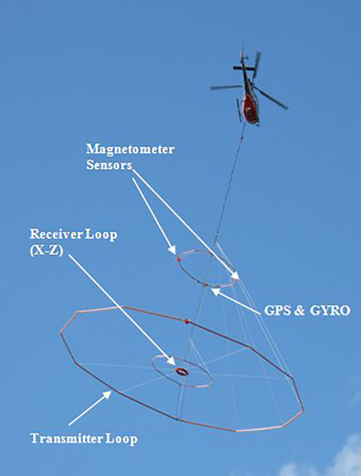
Figure 1: Horizontal Gradiometer (HGrad) system mounted on a VTEM platform.
Horizontal Gradiometer (HGRAD) System Descriptions
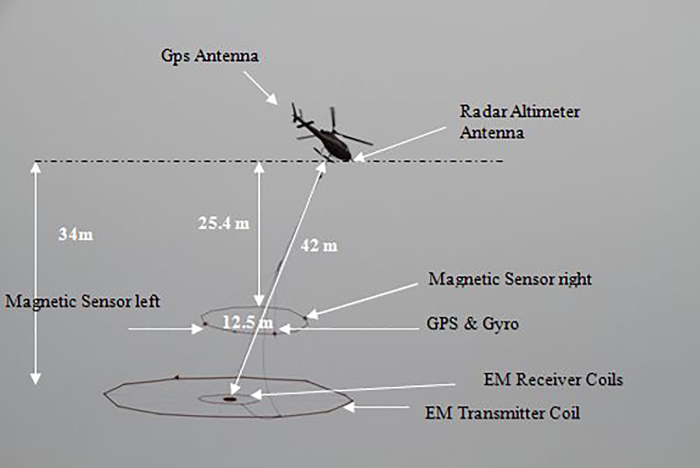
Figure 2: VTEM horizontal gradiometer configuration and dimensions.
In Figure 2, the VTEM horizontal gradiometer in full flight configuration and its relevant dimensions are shown. The horizontal gradiometer loop is mounted about 10m above the VTEM transmitter coil. The nominal diameter of the flexible loop is 12.5m. During survey flight, the gradiometer loop can sway or tilt due to different wind conditions. Therefore, it is essential to have a GPS receiver and a Gyro Inclinometer to record the position and orientation of the gradiometer at all times. The information will be used in subsequent magnetic data corrections.
Magnetic Data Corrections
The magnetic data collected from a horizontal gradiometer (HGrad) system are corrected for spikes and diurnal variations. No lag correction is needed for the magnetic data, since the position of bird GPS receiver is used as the data coordinate.
However, some special corrections pertinent to gradiometer systems only must be applied to the data collected from the VTEM horizontal gradiometer and HeliGrad. Those corrections will be discussed in the following sections.
Corrections Applied to VTEM Horizontal Gradiometer Data
The positions of the two magnetic sensors are determined from the GPS and Gyro data from the magnetic loop.
The first correction applied to the magnetic data is the height correction. The height differences of the sensors with respect to the horizontal plane, which passes through the mid-point the vertical positions of the sensors, are calculated. The magnetic data are either upward or downward continued to the ideal horizontal plane, Figure 3.
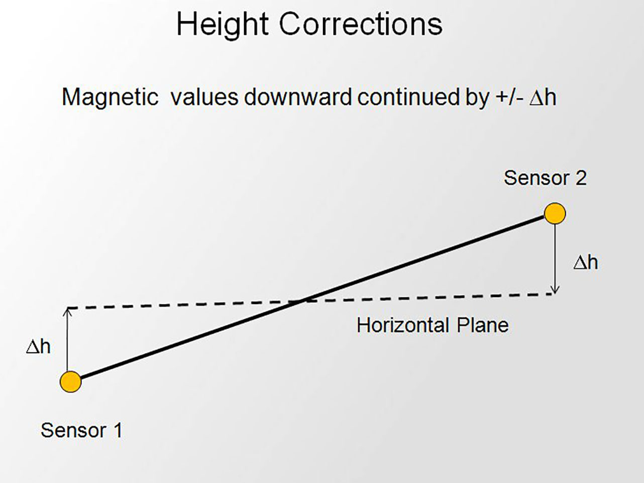
Figure 3: Height corrections applied to VTEM Horizontal Gradiometer data.
The second correction applies to the measured horizontal gradient vectors if they deviate from the ideal longitudinal and lateral axes due to rotation around the vertical axis. This correction simply projects the horizontal gradients to the ideal axes, Figure 4.
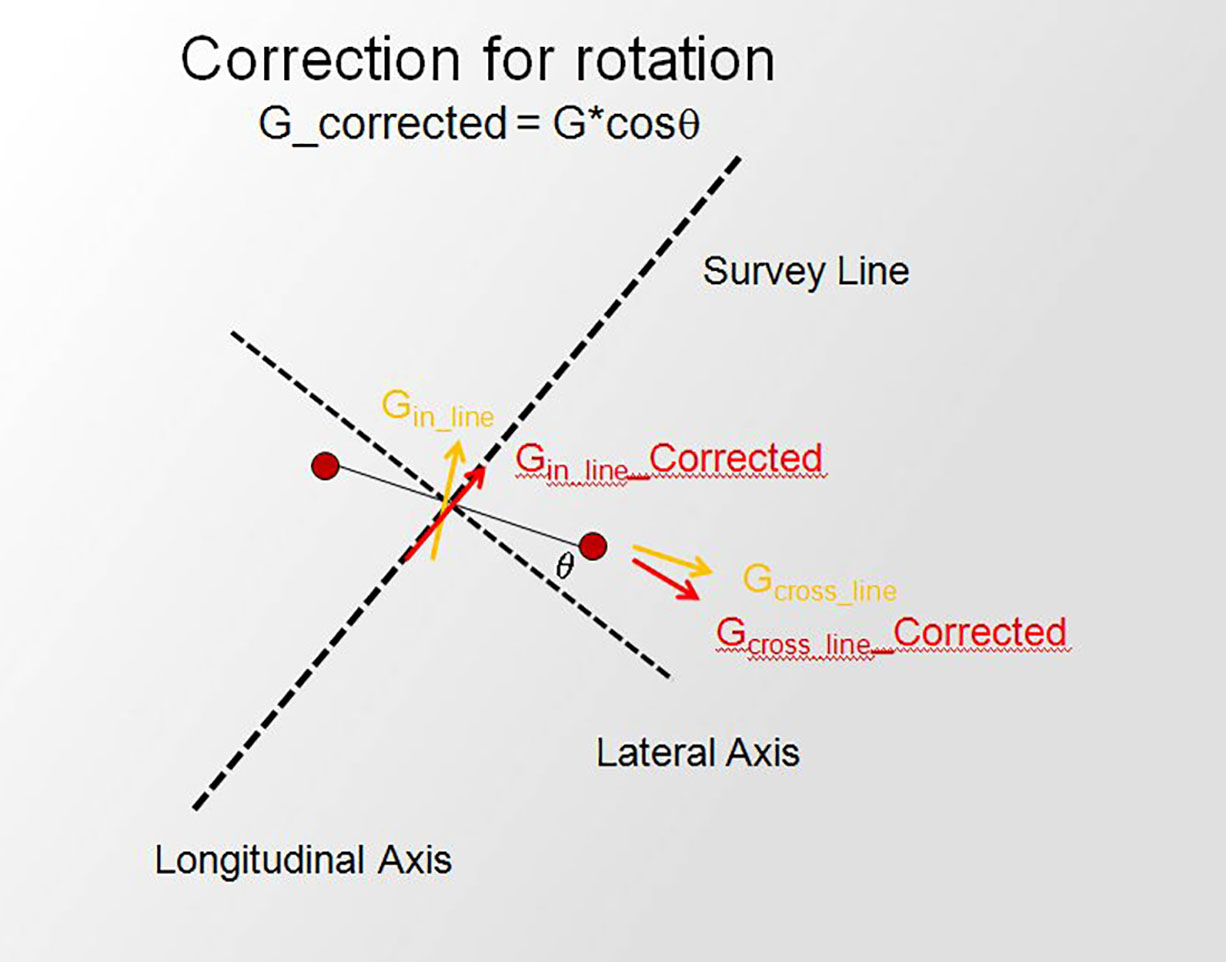
Figure 4: Rotational correction applied to VTEM Horizontal Gradiometer data.
Measured Vs. Calculated Gradients
One can calculate gradients from Total Magnetic Intensity (TMI) data collected using a single magnetometer by 1D FFT for in-line and vertical gradients and 2D FFT for cross-line gradient. Under normal circumstances, the calculated in-line and vertical gradients are fairly comparable to the measured ones, except for very active magnetic areas. However, for cross-line gradient, the calculated is much inferior to the measured, as shown in Figure 5.
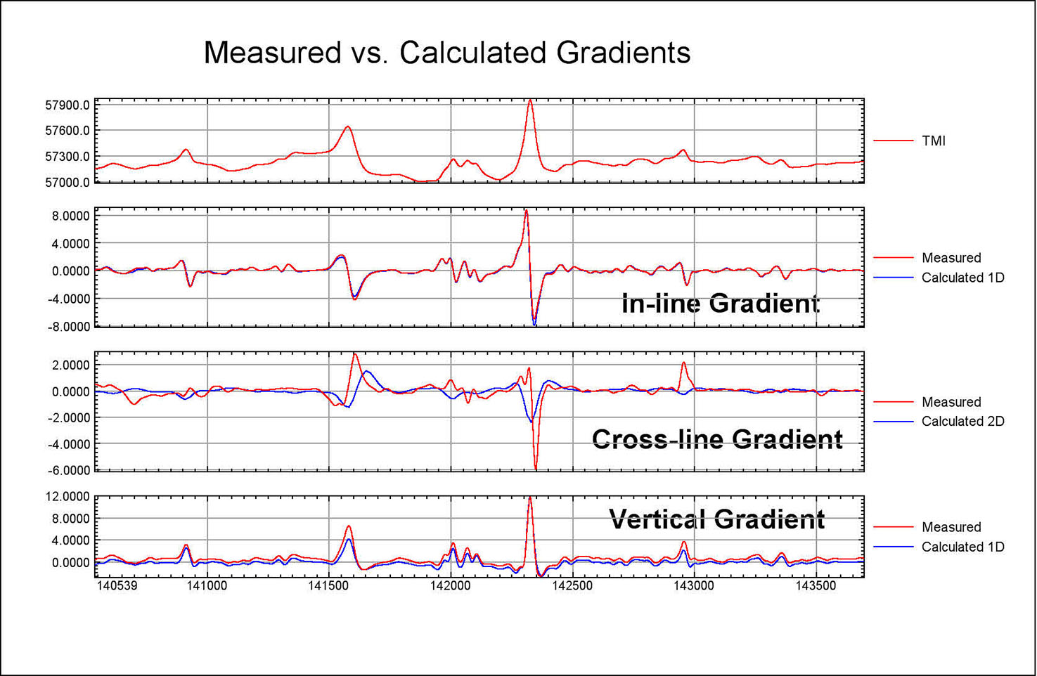
Figure 5: Comparison of Measured and Calculated Gradients, HeliGrad system.
Field Data from a Horizontal Gradiometer (HGRAD) System
For a VTEM horizontal gradiometer (HGrad) system, only the cross-line gradient data are measured. The in-line gradient can be calculated using 1D FFT or the first difference of two consecutive measurements divided by interval length. The vertical gradient is computed using 1D FFT. Total Magnetic Intensity (TMI) values are taken as the average of the TMIs from the two magnetometers.
Field data collected by a horizontal gradiometer system in Flin Flon VMS district in Manitoba, Figure 6, are used to demonstrate the quality and utility of the magnetic gradient data. The survey was flown at N143oE nominal line direction and 160m nominal line spacing. The survey was commissioned by Quantum Minerals Corporation, as part of the Namew Lake and Rocky Lake exploration projects.
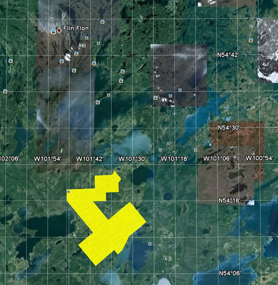
Figure 6: VTEM with horizontal gradiometer survey location .
The general geology of the area consist Early Proterozoic gneisses under the sedimentary cover. Metavolcanics, metasediments and orthgneisses show early isoclinal folding (fold limps are parallel) and later arching and doming. The folding structures in some areas are too small and complex to be resolved by a single magnetometer survey. Therefore, a VTEM combined with a horizontal magnetic gradiometer survey is a rather sensible approach to current exploration problem.
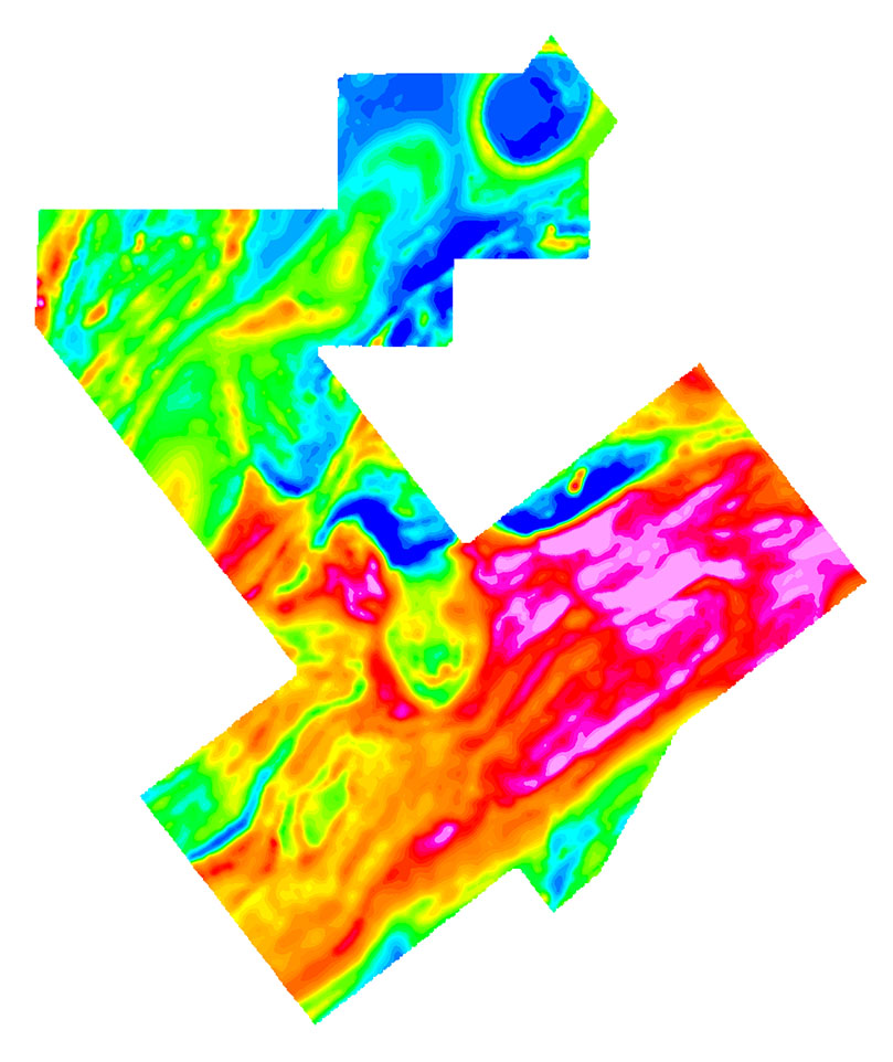
Figure 7: TMI data.
In Figure 7, the TMI data are displayed. The folding structures, isoclinal, doming and arching folds, can be seen in the TMI, but without the fine details.
Advanced derivatives, such as the total horizontal gradient, tilt-angle derivative, can be derived from the measured cross-line and calculated in-line and vertical gradients. The total horizontal gradient ∂M/∂h , and tilt-angle q derivative, are defined below (Salem 2008):
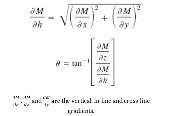
The derived total horizontal gradient and tilt-angle derivative are shown in Figure 8. These two advanced gradient products provide even greater details in the magnetics for interpretations of fold axes and faults, Figure 9.
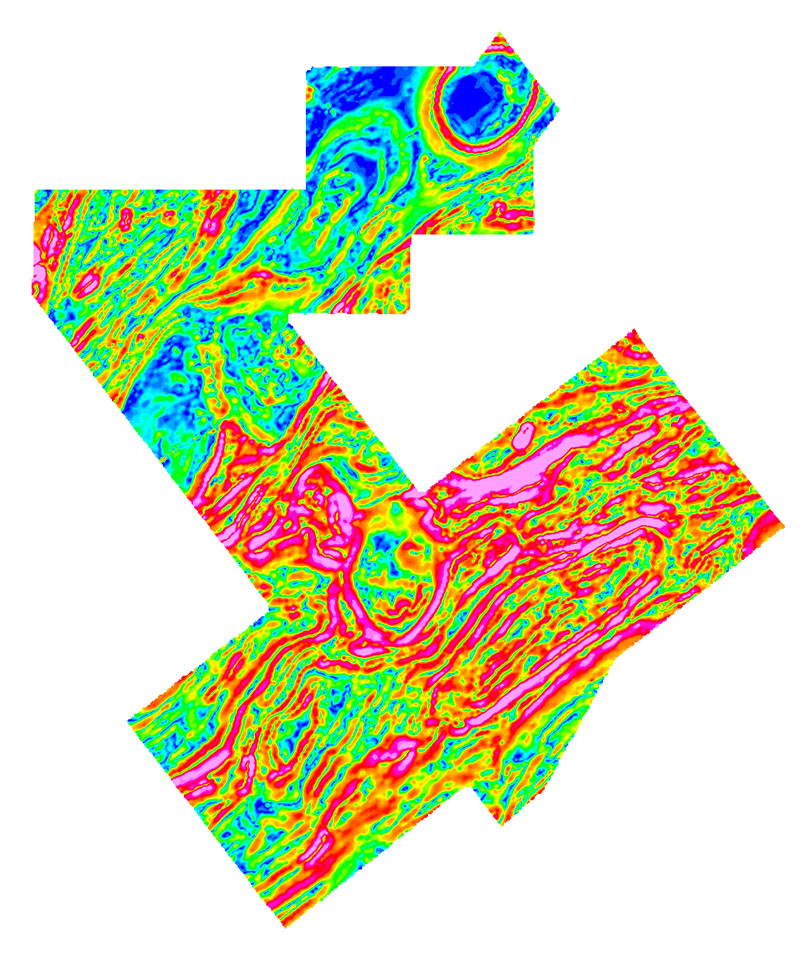
Figure 8: Calculated total horizontal gradient.
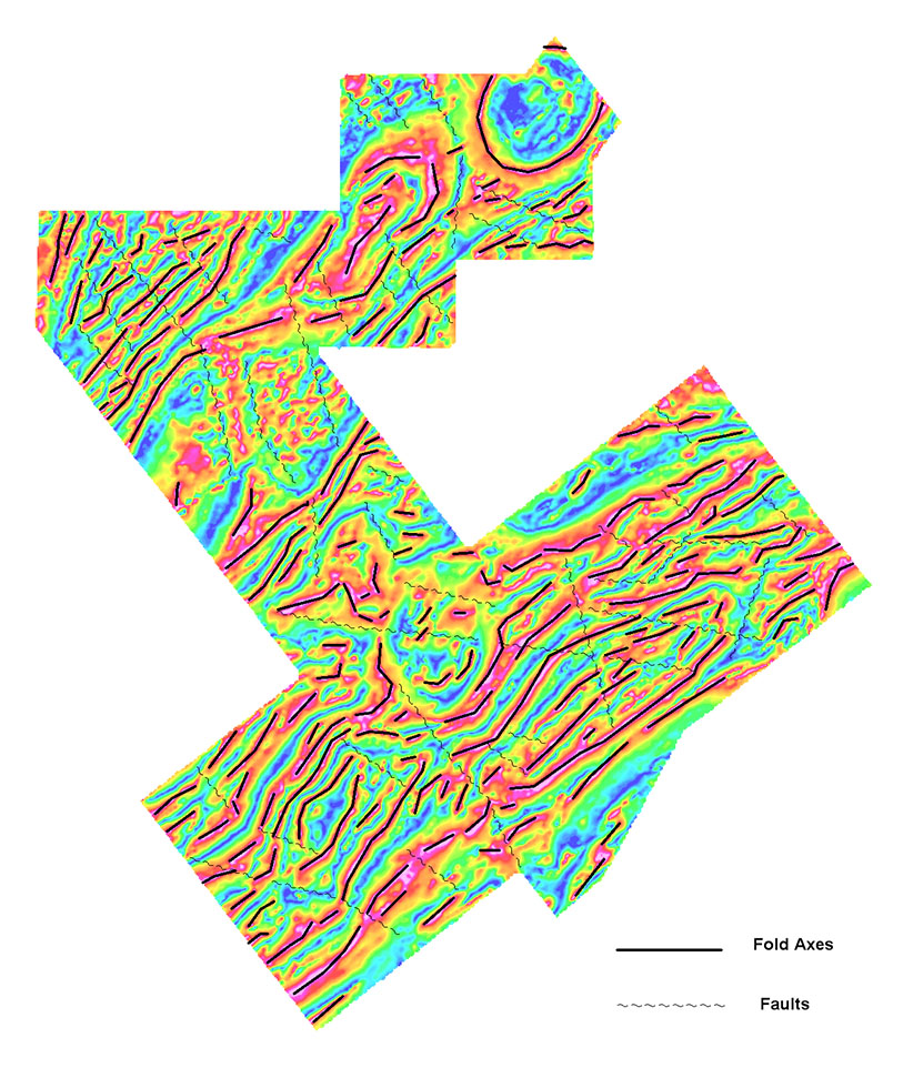
Figure 9: structural interpretations of fold axes and faults overlain tilt-angle derivatives.
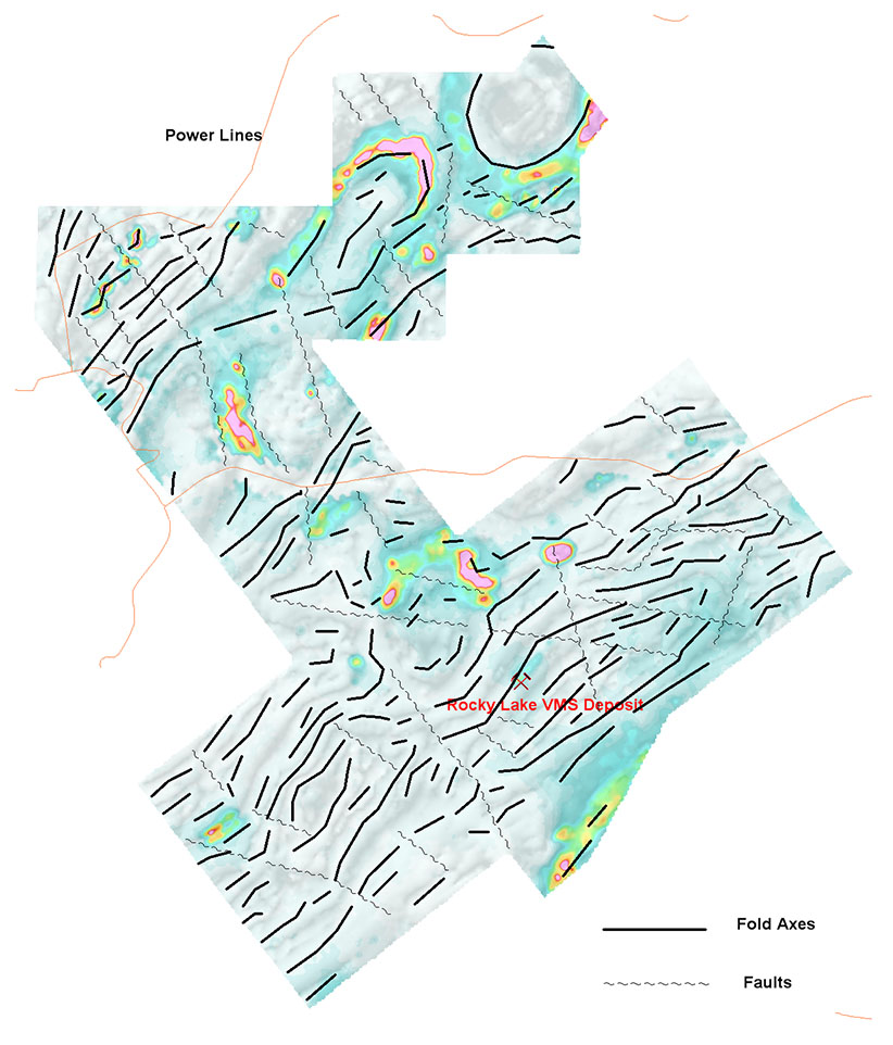
Figure 10: Time constant TAU (color) over Tilt derivative (gray) with structural interpretations and Rocky Lake VMS deposit.
In Figure 10, the time constant TAU computed for VTEM data are displayed, along with the interpreted fold axes and fault. Together with the tilt derivative in the background (in gray), it is quite obvious that the conductors (high TAU values) are located either on or near fold axes and faults. For example, the Rocky Lake VMS deposit is located along a major fold limp and on a moderate to high TAU anomaly.
Conclusions
The horizontal gradiometer (HGrad) system mounted on the VTEM platform provides high-resolution measured cross-line magnetic gradient data. The gradient data are corrected for distortions due to sensors height and rotation variations. The measured cross-line gradient data collected by the HGrad system, along with the calculated in-line and vertical gradients, can be used to compute the total horizontal gradient and tilt-angle derivative. All gradients and advanced derivatives offer greater details in the magnetics for structural interpretations. Together with VTEM data, potential VMS targets can easily spotted and interpreted.
Acknowledgements
We would like to express our gratitude and thanks to Quantum Minerals Corporation for permission to use the VTEM and horizontal gradients data in this presentation.
References
Hardwick, C.D., 1999, Gradient-enhanced total field gridding: Expanded abstracts, SEG Houston, Gravity and Magnetics, 2.7
Reford, Stephen, 2004, Gradient enhancement of the total magnetic field, SEG AGM, Magnetic Gradiometry Workshop, Expanded Abstracts, GM P1.1
Reid, A. B., Allsop, J. M., Granser, H., Millet, A.J. and Somerton, I. W., 1990, Magnetic interpretation in three dimensions using Euler deconvolution, Geophysics, Vol.55, pp.80-91.
Salem, A. et al, 2008, Interpretation of magnetic data using tilt-angle derivatives, Geophysics, vol. 73, no. 1, p.L1-10.
Thurston, J.B. and Smith, R.S., 1997, Automatic conversion of magnetic data to depth, dip, and susceptibility contrast using the SPITM method, Geophysics, Vol.62, pp.807-813.