For a PDF of this paper click here
Introduction
December 11 to 12, Geotech had flown some test lines near Saint-Hyacinthe, Quebec, using the VTEM early time system, figures below. Some test lines coincide with ground TEM data locations. The ground TEM data were inverted using the Laterally Constrained Inversion (LCI) technique. VTEM data were inverted using Geotech Heuristically and Laterally Constrained Inversions (HLCI).
In the following sections, the results of LCI of ground TEM data and HLCI of VTEM data, when their locations coincide, are presented. Those VTEM lines include L1000, parts of L1001, L5000 and L6000. L5000 VTEM data were difficult to invert because it was flown over several power lines.
L2000 is a very long test line, and it was flown over several power lines as well. Two segments of the line, free of power line influences, was selected for HLCI.
L7000 were flown over several power lines, so HLCI was not attempted.
The below table summarizes VTEM test line status and HLCI.
| Line | Major Power Lines | HLCI | Ground TEM coverage |
| 1000 | 0 | Yes | Full |
| 1001 | 1 | Yes | Partial |
| 6000 | 3 | Yes | Full |
| 5000 | 4 | Yes | Full |
| 2000 | 5 | Yes | None |
| 7000 | 2 | No | None |
Geology
Local lithology consists of, approximately, a 20-70m thick layer of clay, with resistivity ranging from 5 to 60 ohm-m, overlying fractured rock partially saturated with saline water.
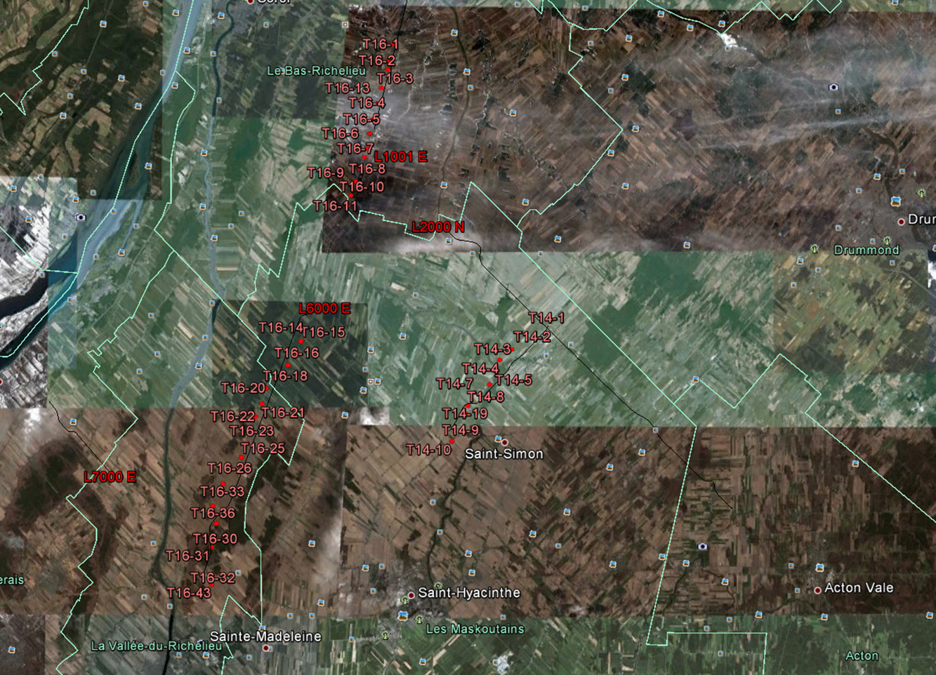
Figure 1:VTEM test lines locations (black lines); Red dots are Ground EM locations.
Heuristically and Laterally Constrained Inversion (HLCI)
HLCI is a pseudo 2D layered earth inversion algorithm developed by Geotech LTD. HLCI is built on Airbeo (CSIRO/AMIRA), a layered earth 1D inversion package developed by Commonwealth Scientific and Industrial Research Organization (CSIRO) over the span of 25 years. The package, along with its FORTRAN source codes, was released to the public in 2007.
HLCI consists of two phases, I and II. In Phase I, normal Airbeo 1D inversions, with a single initial model, are run for all VTEM readings. After that, the inversions are evaluated. Also, lateral constraints are built based on the layer depths computed in Phase I. The lateral constraints, which minimize the layered earth structures along the in-line horizontal direction, are the results of statistical mean filtering. The filter length is user-defined, by trial-and-error or experiment (hence the word heuristically being used here). Filter length can be influenced strongly by geology. A priori information, such as drillhole derived layer depth, can be used at this stage to better define the lateral constraints.
In Phase II, Airbeo is run for all VTEM readings again. But this time, different initial models with fixed layer depths, which are laterally constrained by neighboring models, are used in the inversions. The inversion outputs are laterally consistent in terms of layer depths. Layer resistivities can be filtered by a user designed filter afterwards too.
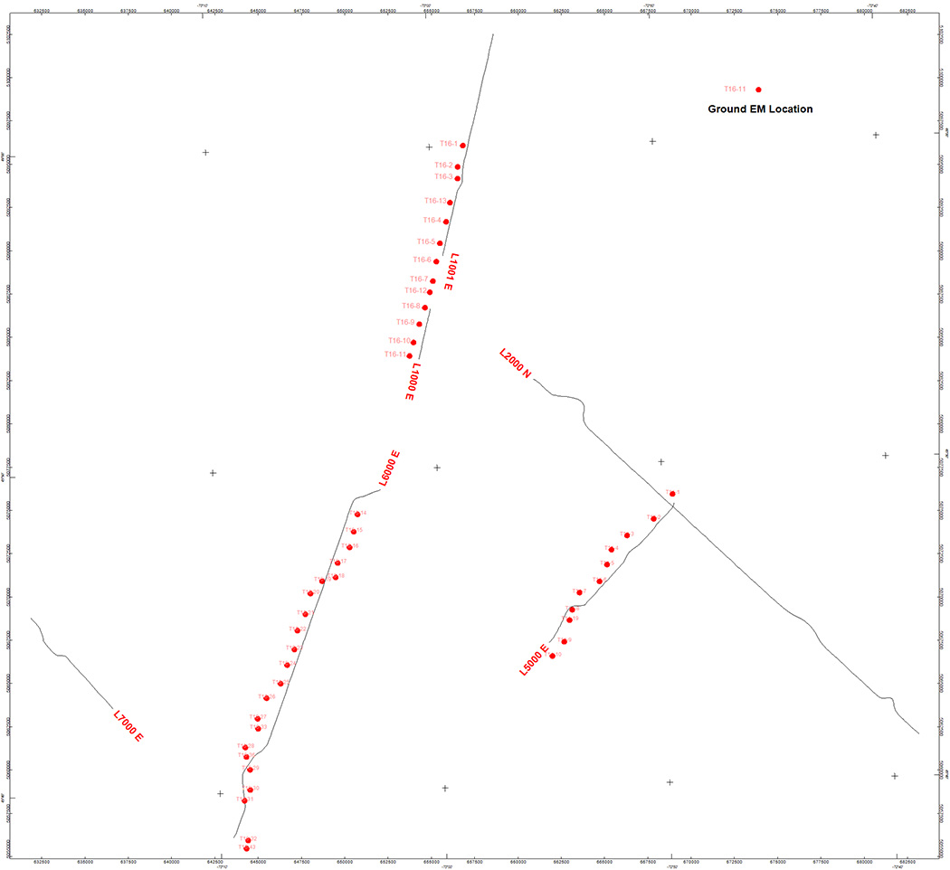
Figure 2:VTEM test lines and Ground EM locations.
L1000 and L1001
Parts of L1001 have ground TEM coverage, and they are merged with L1000 for HLCI. HLCI for entire L1001 will be presented later.
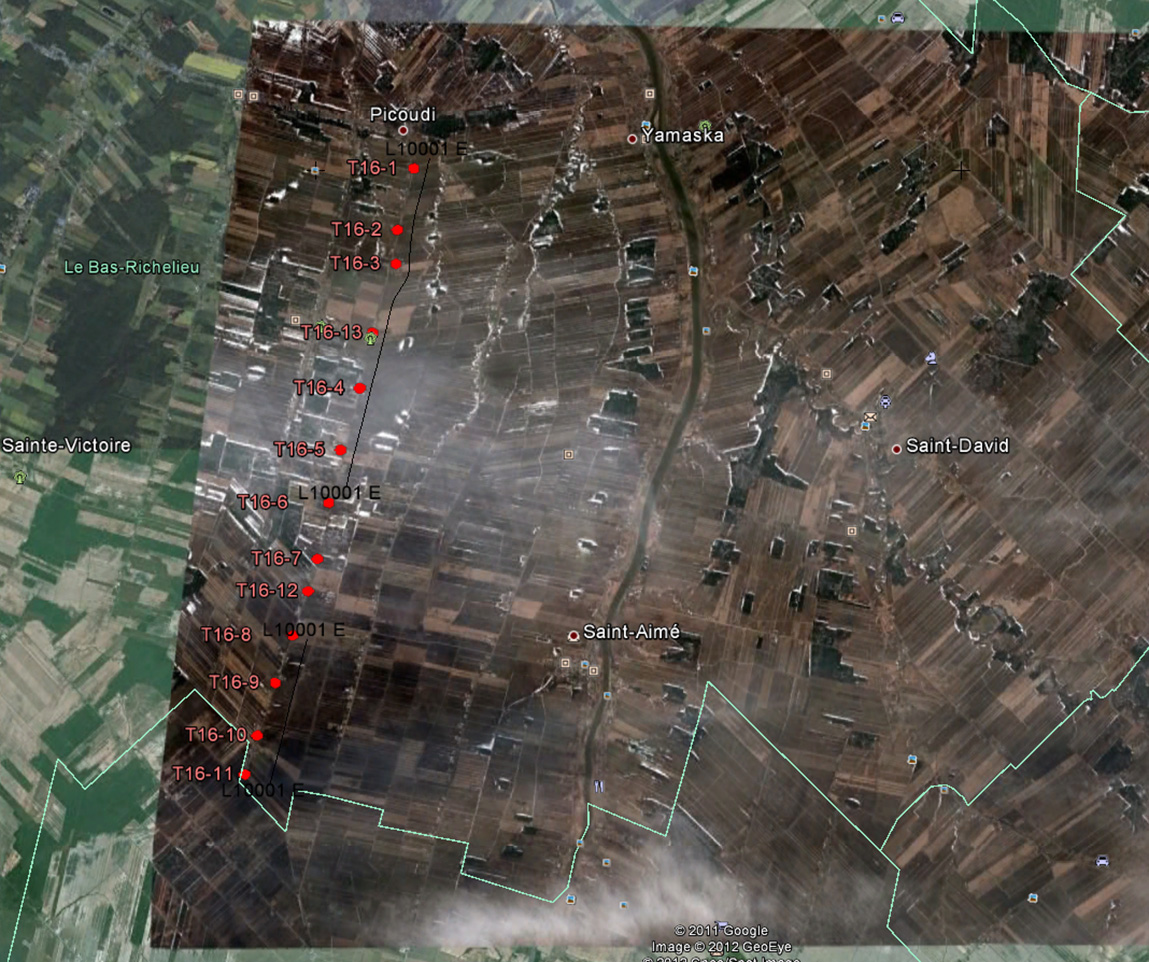
Figure 3:Locations of ground TEM and VTEM lines.
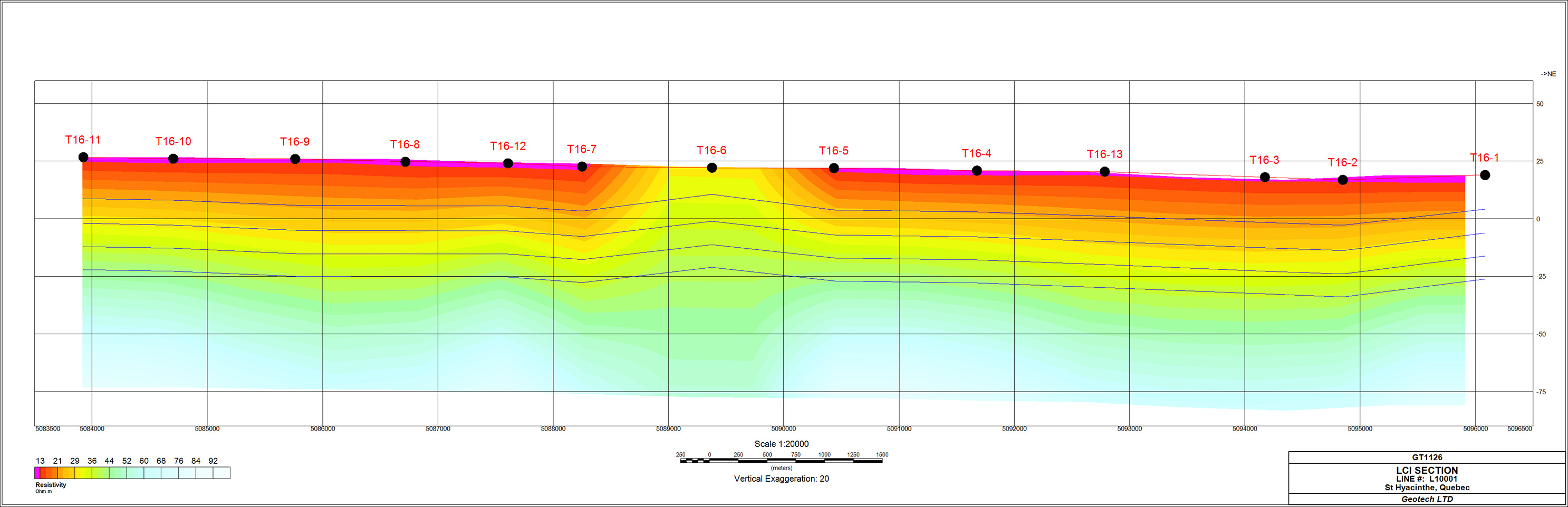
Figure 4:LCI of ground TEM data; layer depths are plotted (blue lines).
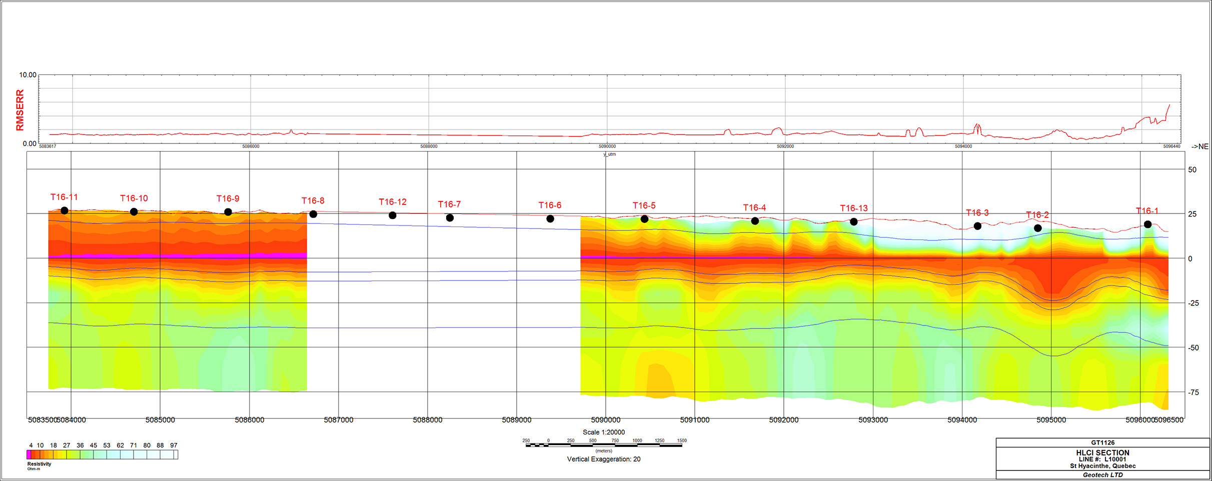
Figure 5:HLCI of VTEM data, top panel shows the RMS errors and layer depths are shown by blue lines.
Figure 4 and 5 Comparisons
• Same color scale is used for both sections;
• Both show a conductive layer (probably the clay layer) near surface.
• HLCI of VTEM shows more structures (saline water in fractured rocks) at depth below the conductive layer, as well as a thin resistive layer to the north.
L6000
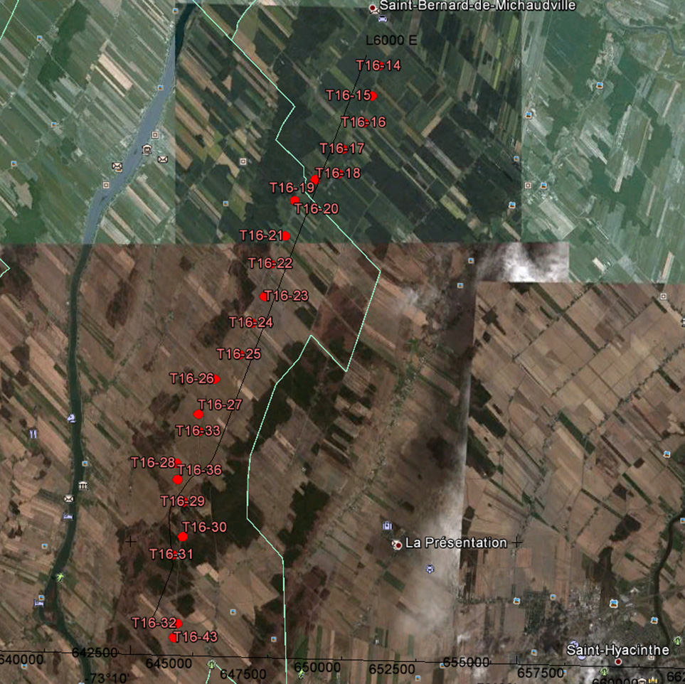
Figure 6: Location.
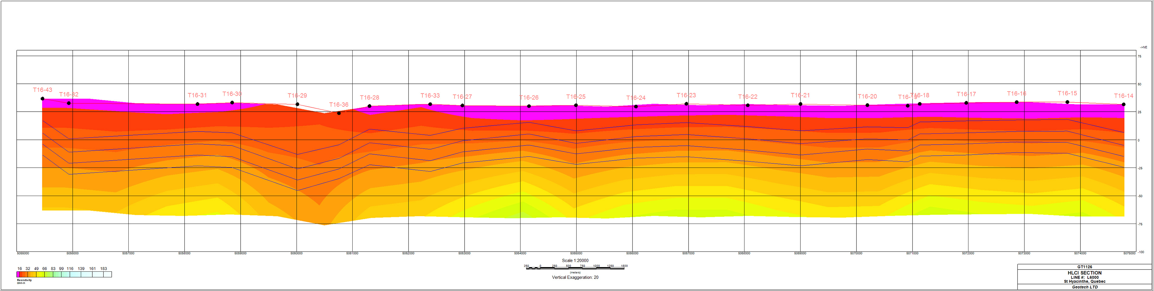
Figure 7:L6000 LCI of ground EM, layer depths shown as blue lines.
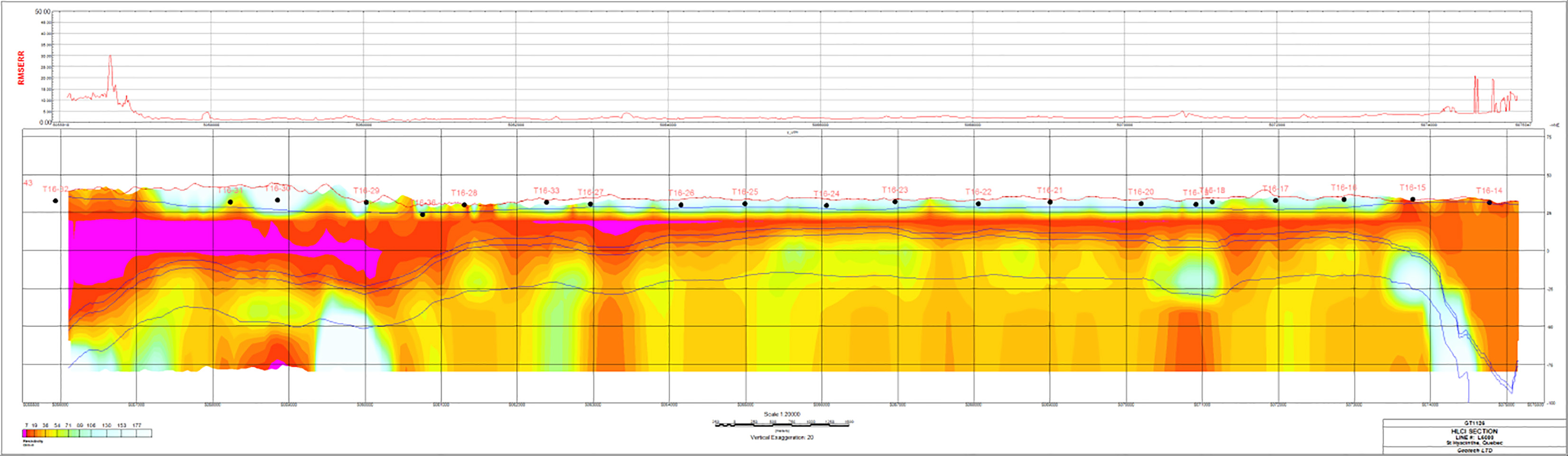
Figure 8: L6000 HLCI of VTEM, layer depths shown as blue lines; top panel shows RMS errors.
Figure 7 and 8 Comparisons
• Same color scale is used for both sections;
• Both show a conductive layer (clay) near surface:
• There is a major power line near the southern end of the line, figure below.
• HLCI of VTEM shows more structures at depth below the clay layer (saline water in fractured rocks), as well as a thin resistive layer to the north. There is a steeply dipping resistive layer near the north end.
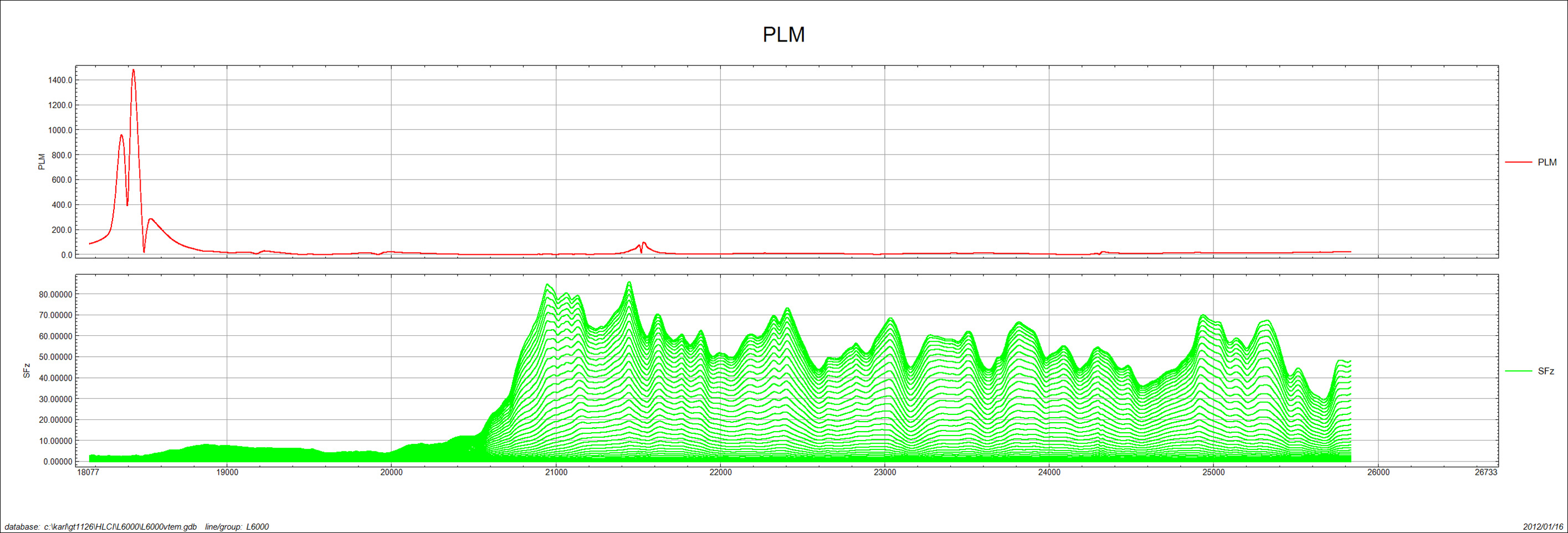
Figure 9:Power Line Monitor (PLM) and VTEM dB/dt Z component data.
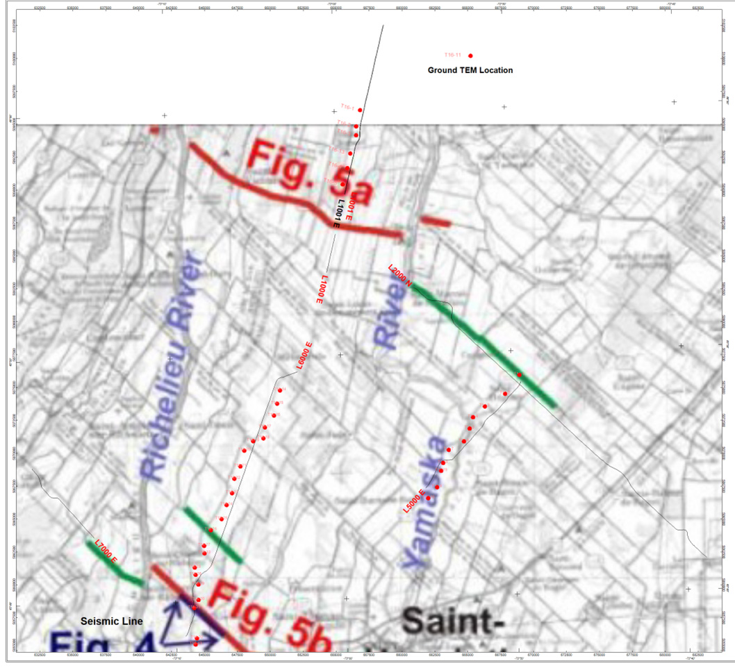
Figure 10: The southern end of L6000 intersect a seismic line from (Pugin, Andre J-M., et al, 2011, seismic reflection surveying in regional hydrology: an example from the Monteregie region, Quebec, Geological survey of Canada).
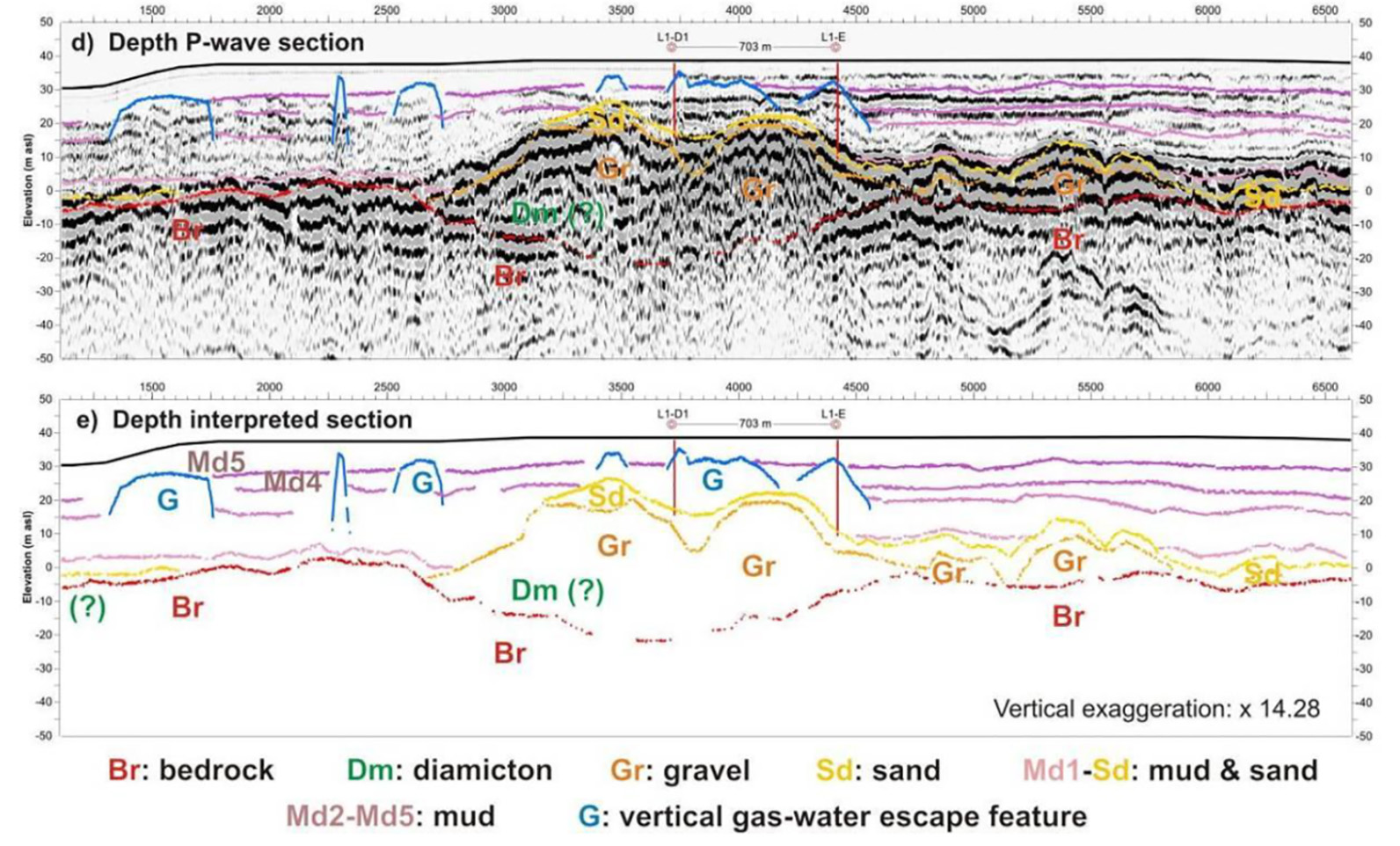
Figure 11: The seismic section and the interpretations are shown in the figure above (sections displayed from NW to SE). As we can see, the bedrock is about 25-30m below the surface. Unfortunately, the VTEM data near the southern end of L6000 are heavily contaminated by power line signals.
L5000
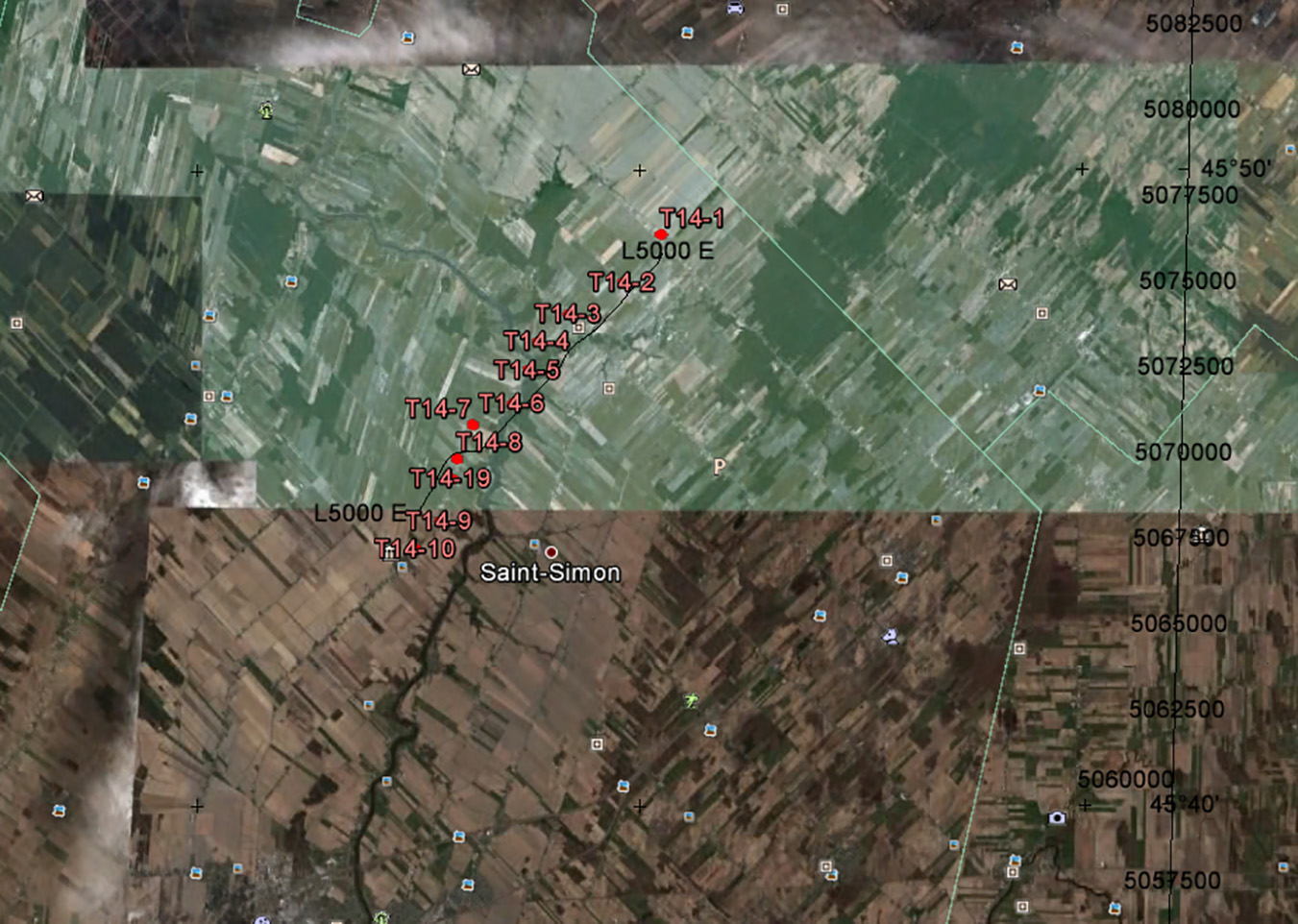
Figure 12: Location.
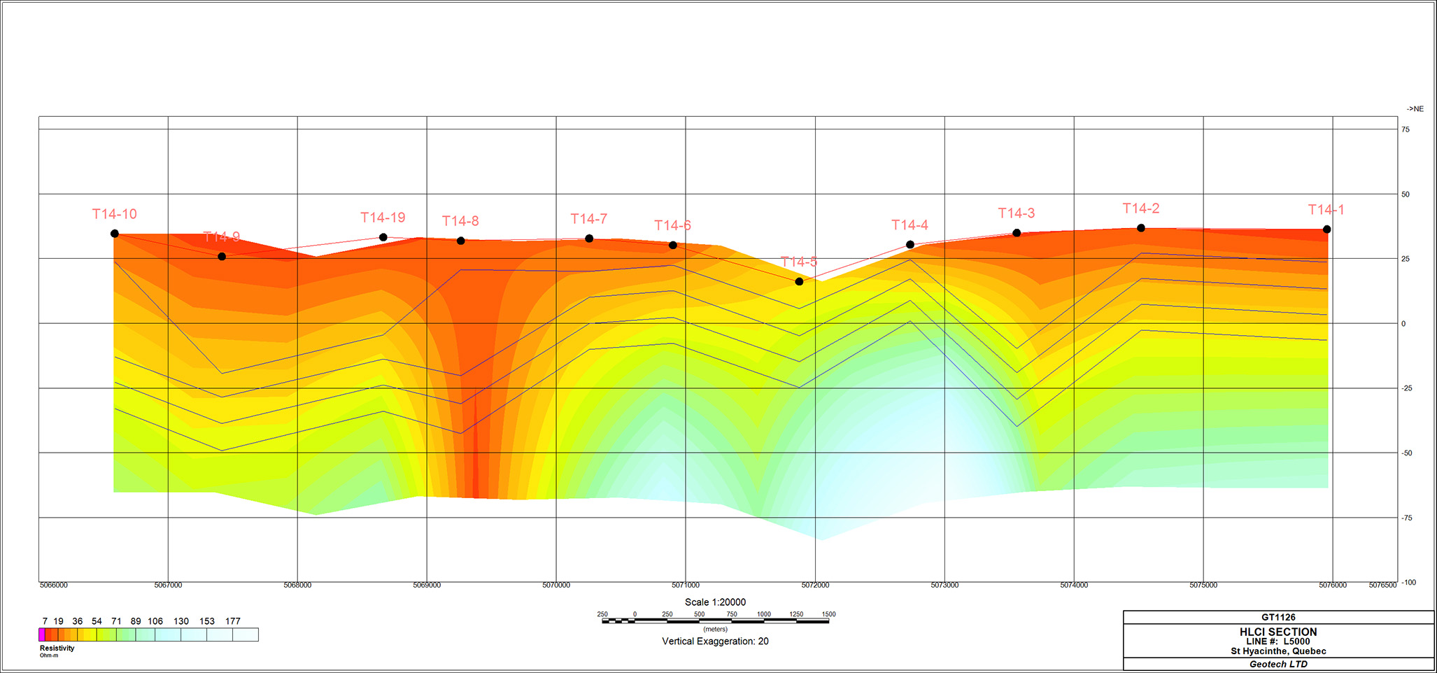
Figure 13: LCI of ground EM, maximum depth displayed is 100m.
Figure 14: HLCI of VTEM data, maximum depth displayed is 200m.
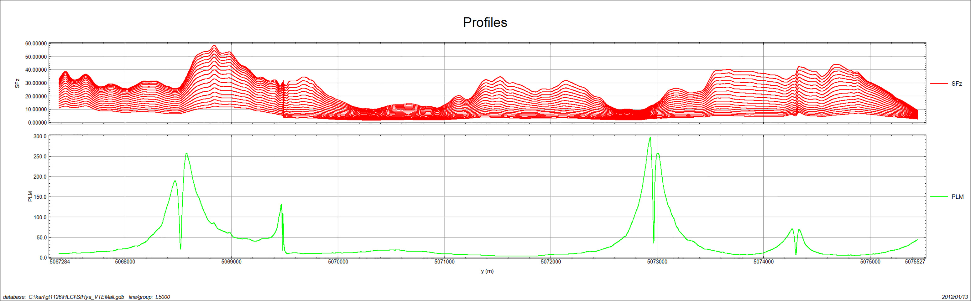
Figure 15: VTEM dB/dt Z (SFz) and Power Line Monitor (PLM) profiles.
Comparisons
• Same color scale is used for both sections;
• HLCI of VTEM data have large RMS errors in some places.
• Both show a large, near vertical conductive body in the south.
• This line is under the influences of at least three power lines! As a result, inversions are very difficult to interpret.
Summary
Both LCI of Ground TEM and HLCI of VTEM show a shallow conductive layer, probably corresponding to the clay layer, for Line 1000, 1001 and 6000. For L5000, the case for layered earth is hampered by strong interferences from the power lines.
LCI of Ground TEM shows the clay layer near the surface, but little details above and below the layer. HLCI of VTEM data are able to show a more complete structure above and below the clay layer. This is not surprising, since VTEM data are sampled at approximately 3m interval. Ground TEM cannot match VTEM’s data density.
L1001
Figure 16: L1001 location.
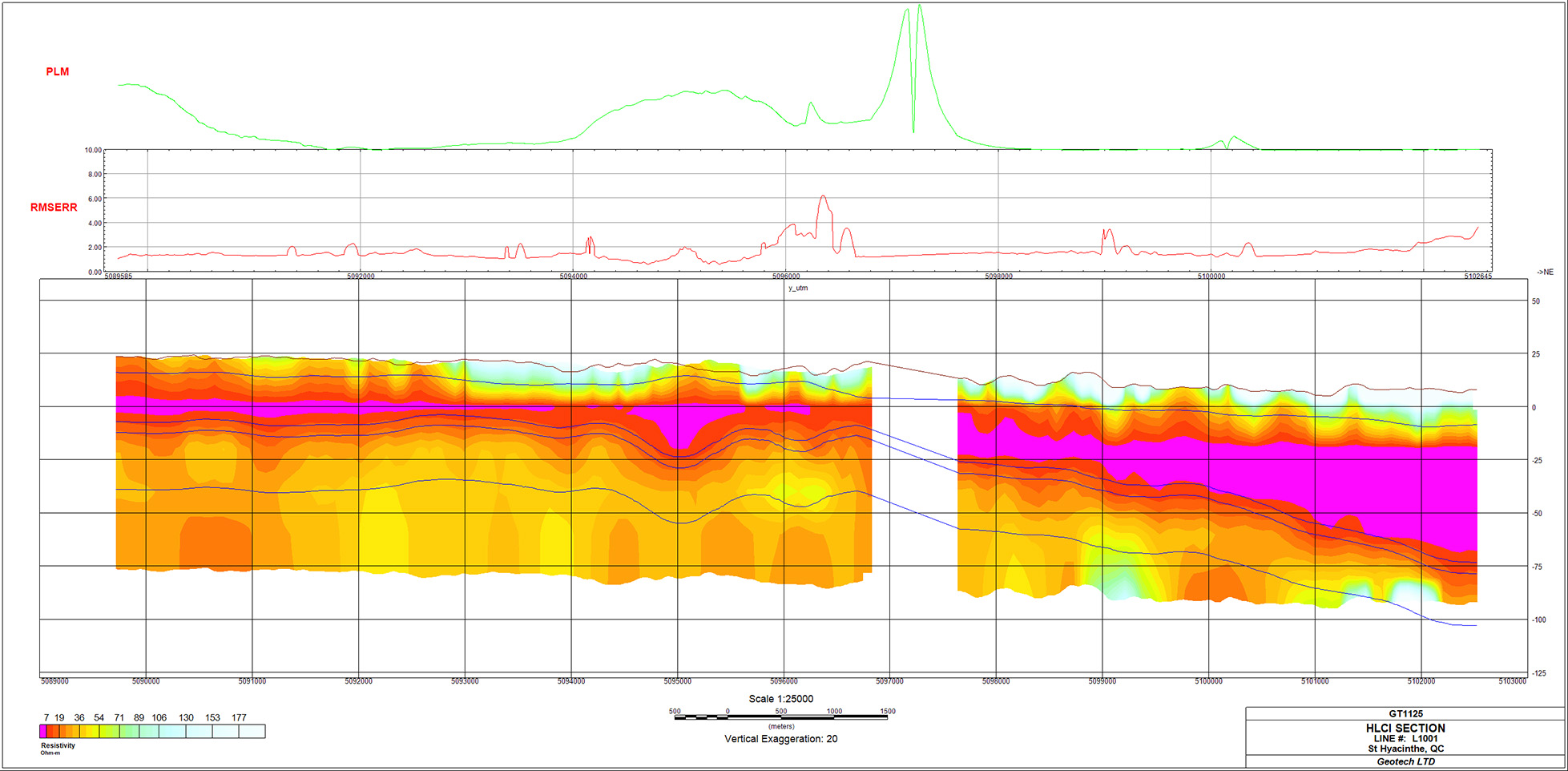
Figure 17: HLCI of VTEM data; top panels show Power Line Monitor and RMS Errors respectively.
Interpretations
The conductive clay layer is seen quite clearly in the HLCI section plot. The clay layer increases its thickness from south to north. There is a thin resistive layer above the clay. Below the clay layer, the conductivities are moderate, and the structures are not layered but sub-vertical instead.
L2000 – Part I
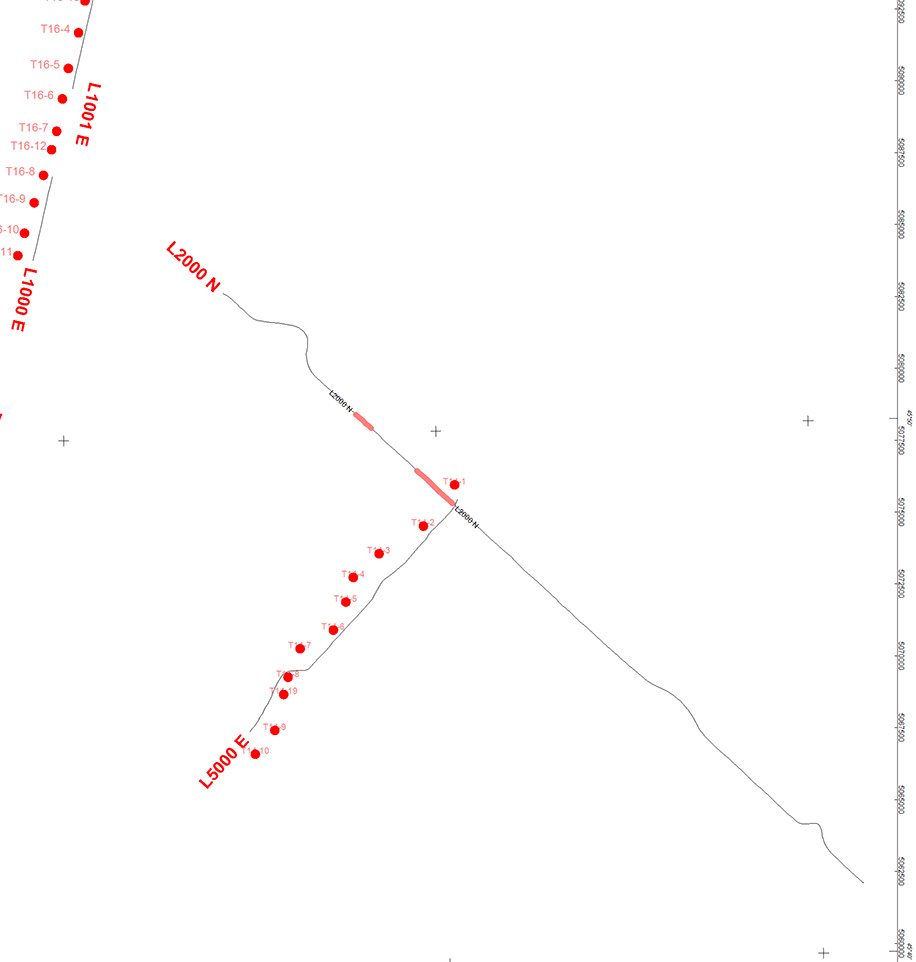
Figure 18: Location; two selected segments from L2000, avoiding the worst of power lines.
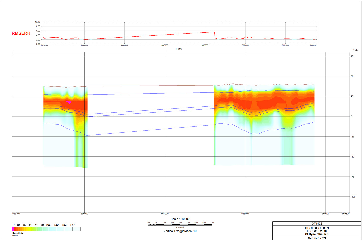
Figure 19: HLCI of VTEM.
Interpretations
HLCI of VTEM data for the two small segments from L2000 show the clay layer quite well. The units above and below the clay are relatively resistive.
L2000 – Part II
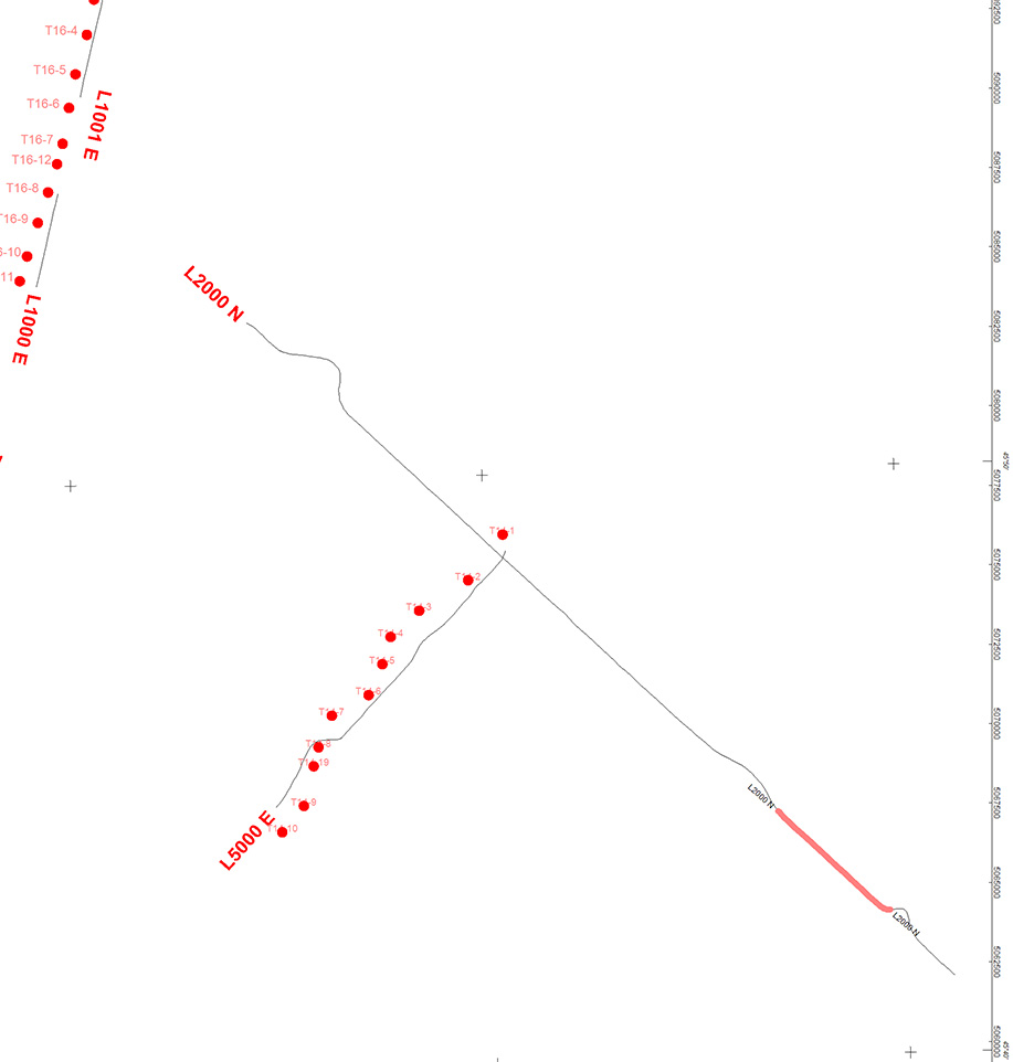
Figure 20: Location
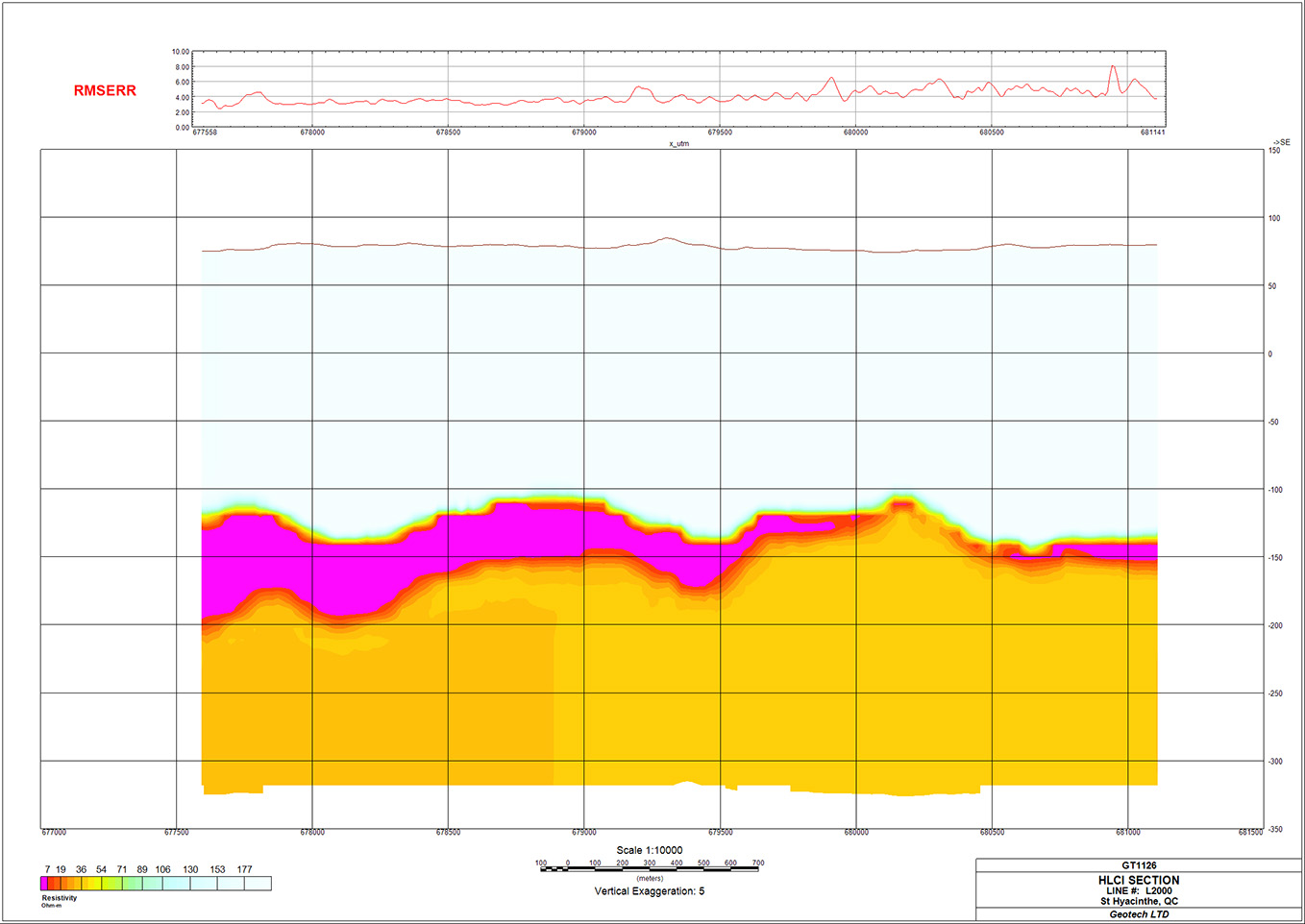
Figure 21: HLCI of VTEM.
The VTEM data come from the far Eastern end of L2000. HLCI show a conductive layer, unknown lithology, almost two hundred meters below surface. The layer pinches out to the east. Above the conductive layer, the unit is relatively resistive. Below the clay, the unit is relatively conductive.