Presented at SAGEEP 2014
For a PDF of this paper click here
Abstract
The performance of two-dimensional (2-D) joint ZTEM™/MT inversion was tested using synthetic brick structures below a hill and valley model. Subsequently, separate and joint inversion of coincident ZTEM and Titan dense array MT data over the Johnston Lake district, Saskatchewan, were performed. A result of this effort is that only very few (e.g., three) MT stations may be needed to correct for background resistivity effects in a ZTEM survey provided the MT sites are appropriately spaced.
Introduction
Audio Frequency Magnetic (AFMAG; Ward, 1959; Labson et al., 1985) is an electromagnetic prospecting method where naturally propagated EM fields originating with regional and global lightning discharges (sferics) are measured as a means of inferring subsurface electrical resistivity structure. A helicopter-borne coil platform (bird) measuring the vertical component of magnetic (H) field variations along a flown profile is referenced to a pair of horizontal coils at a fixed location on the ground in order to estimate a tensor H-field transfer function.
The ZTEM method is distinct from the traditional magnetotelluric (MT) method in that the electric fields are not considered because of the technological challenge of measuring E-fields in the dielectric air medium. This can lend some non-uniqueness to ZTEM interpretation because a range of conductivity structures in the earth depending upon an assumed average or background earth resistivity model can fit ZTEM data to within tolerance. MT data do not suffer this particular problem, but they are cumbersome to acquire in their need for land-based transport often in near-roadless areas and for laying out and digging in E-field bipole sensors. The complementary nature of ZTEM and MT logistics and resolution have motivated development of schemes to acquire appropriate amounts of each data type in a single survey and to produce an earth image through joint inversion. In particular, consideration is given to surveys where only sparse MT soundings are needed to drastically reduce the non-uniqueness associated with background uncertainty while straining logistics minimally.
Other workers (Holtham and Oldenburg, 2010; Sasaki, 2013) have presented joint 3D inversion studies using sparse but regularly spaced MT soundings and denser ZTEM measurements. Spratt et al. (2010) analysed inversions of synthetic ZTEM data from 2D MT conductivity models to determine their usefulness in mapping a sedimentary basin. The present study investigates the capability of 2D joint MT-ZTEM inversion using a few, irregularly spaced MT soundings along a ZTEM survey line.
Method
Algorithm ZTMT2DIV is a generalization from previous code AV2Dtopo (Legault et al., 2009) that inverted ZTEM and AirMt data allowing topographic variations and a variable bird height. The performance of two-dimensional (2-D) joint ZTEM/MT inversion by ZTMT2DIV was tested using synthetic brick structures below a hill and valley model, similar to AV2Dtopo. Subsequently, separate and joint inversion of coincident ZTEM and Titan dense array MT data over the Johnston Lake district, Saskatchewan, were performed. A result of this effort is that only very few (e.g., three) MT stations may be needed to correct for background resistivity effects in a ZTEM survey provided the MT sites are appropriately spaced.
The ZTMT2DIV algorithm makes use of the public domain finite element forward problem and inversion parameter sensitivities using reciprocity developed at the University of Utah (Wannamaker et al., 1987; de Lugao and Wannamaker, 1996), together with the regularized Gauss-Newton non-linear parameter step estimate described by Tarantola (1987). The regularization is a simple damping of the spatial slope of the model variation across the section. Inversion parameters expand in both width and thickness versus depth in order to help equalize influence of different regions of the earth model upon the EM response. The models described were run on a quad-core desktop computer with a 3 GHz Intel I7 processor and typically took 20-60 minutes to execute.
Example 1: Hill-Valley Synthetic Topographic Model
For a synthetic test of the ZTMT2DIV inversion capability, we used the topographic model shown in Figure 1. As shown, there are three brick-like conductors under a hill, a flat section, and under a valley. The depth to the top of the body in the center is about four hundred meters. The depths of the other two bodies are such that it is about 400 m to their tops at some point along their overlying topography. ZTEM responses were computed at the six standard operating frequencies (720, 360, 180 90, 45, 40 Hz) and given Gaussian error values of 0.01. The bodies are 50 ohm-m in a 2000 ohm-m host, which allows the body responses to be near their peak values at the lowest frequency. The bird flight profile is draped to the topography at a height of 90 m. Thus we see a 90 m layer of air lying above the highest topo point in the model mesh. There are 75 ZTEM data points at 100 m intervals. In this model there are only 9 MT sites equally spaced between every 8TH ZTEM site. Their frequencies of operation are from 1000 to 1 Hz in quarter decade intervals (13 in all).
To begin, the inversion performance with the starting model background having the correct value of 2000 ohm-m was examined. Model images resulting from inversion of ZTEM-only responses over the hill-valley model with conductors appear in Figure 2. One sees well resolved, smooth representations of the conductors in their correct subsurface locations. The ‘observed’ and computed responses are not plotted but would be visually identical. Model images from separate inversion of MT-only data appear in Figures 3-4 (TM, TE). The contrast for the transverse magnetic (TM) model is quite low as the body depth is comparable to width. In this mode, the response is dominated by the influence of the electric boundary charges whose falloff with depth is rapid. The transverse electric (TE) mode images are much more prominent in keeping with the stronger TE anomalies, but the image in Figure 5 from joint inversion of ZTEM data and the TM mode is in several ways the best resolved of all, showing the most compactness and correct background values elsewhere.
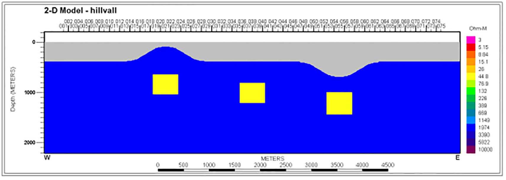
Figure 1: Conductive 50 ohm-m bricks ~400 m deep in resistive 2000 ohm-m half-space under hill and valley used for synthetic test. The gray region is air with 90 m draped bird flight height.
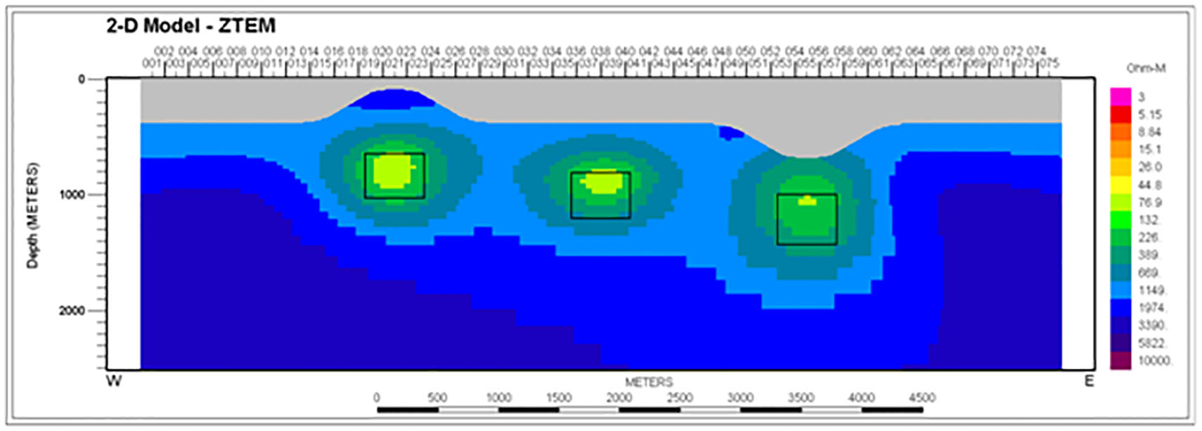
Figure 2: Inversion model of ZTEM response at 6 frequencies from 720 to 30 Hz.
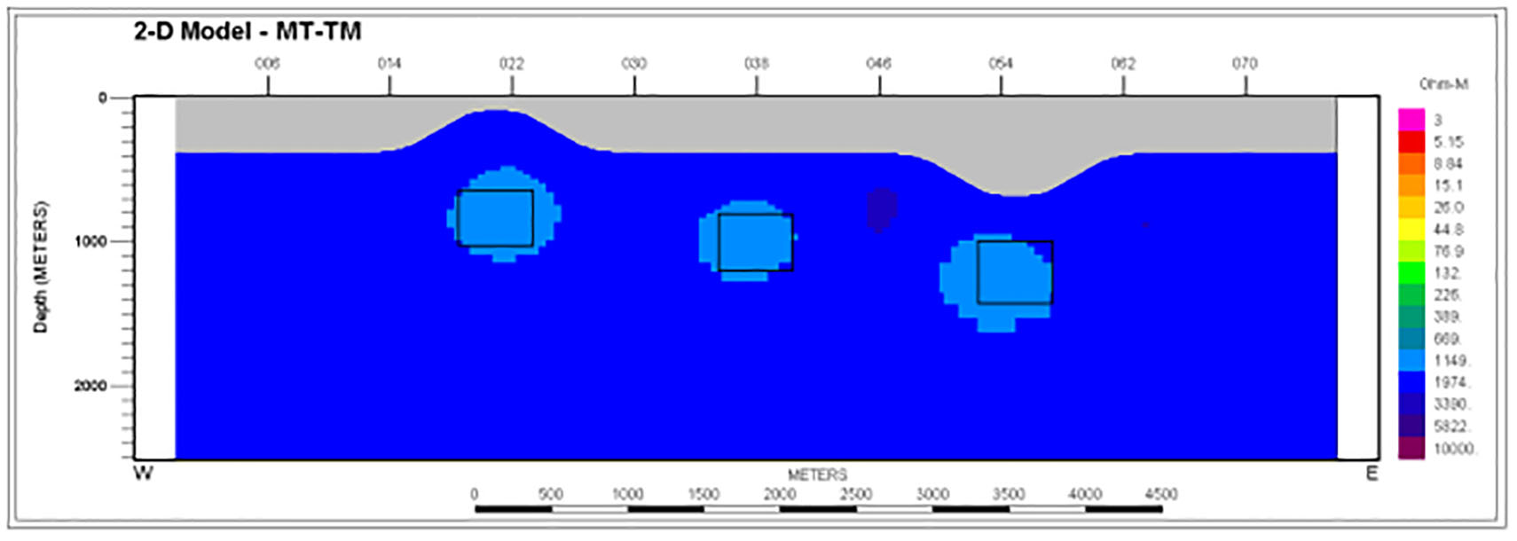
Figure 3: Inversion model of TM mode MT response at 13 frequencies from 1000 to 1 Hz.
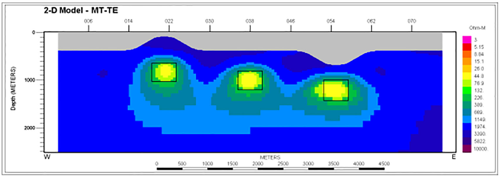
Figure 4: Inversion model of TE model MT response at 13 frequencies from 1000 to 1 Hz.
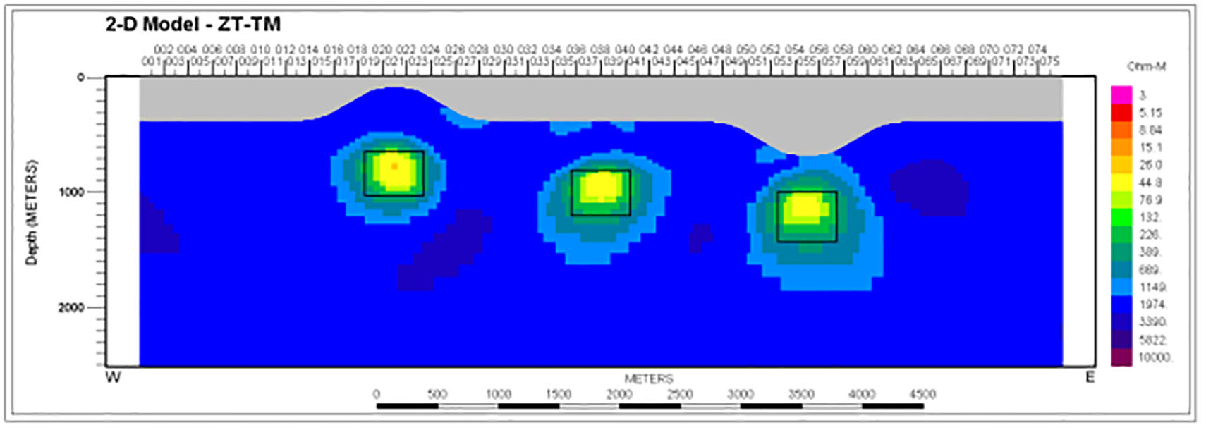
Figure 5: Joint inversion model of ZTEM and TM mode MT responses.
Example 2: Johnston Lake Field Example
A test using measured field data was carried out using coincident ZTEM and Quantec Titan-24 dense MT array profiling from the Johnston Lake unconformity uranium prospect, Athabasca Basin, Saskatchewan. The original ZTEM data profile consisted of 1152 data points over a span of 10027 m. The inversion used just 197 ZTEM locations ~50 m apart for a total span of ~9800 m. The MT profile consisted of 26 continuous sites at 100-150m spacings that extended for 3150 m length over the central third of the ZTEM profile. Thus the MT only spans a fraction of the full length of the ZTEM.
A ZTEM only inversion is plotted in Figure 6 assuming a 2000 ohm-m background. The model shows a compact central conductor in the 1 km depth range and a weak subhorizontal conductor extending southward at somewhat greater depths. A 2D inversion of the TM mode only of the 26 MT sites is shown in Figure 7. This also yielded a central compact conductor though no clear expression of a deeper, weaker one southward. However, the MT data suggest that the background resistivity is greater than previously assumed, more like 4000 ohm-m.
Figure 8 shows a joint inversion of the ZTEM results with the whole TM MT data set. A background of 2000 ohm-m was used. This model shows a strong, compact conductor under the center of the profile with a depth to top <1 km. It extends to depth and then continues southward at a depth >2 km. Note that most of the background increased to ~4000 ohm-m from 2000 with the inclusion of the MT data.
Figure 9 shows a similar joint inversion but with only three MT sites at well-separated but otherwise random positions. This model strongly resembles Figure 8 and a higher resistivity background is recovered as well. This is quite encouraging and supports the previous synthetic study that only a very few MT sites may be required to greatly improve background constraints and improve image accuracy.
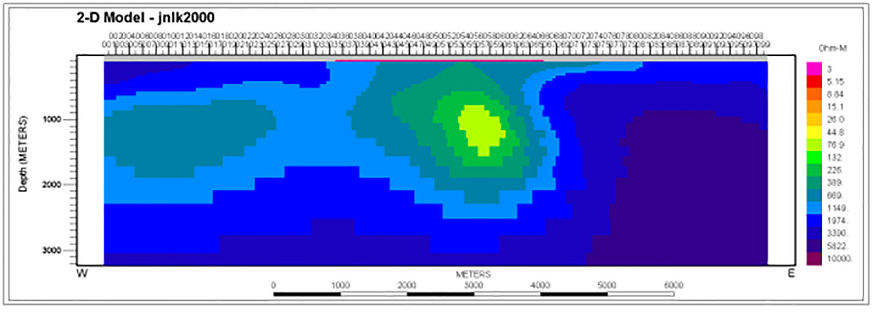
Figure 6: 2D inversion model of 197 binned ZTEM sites along the Johnston Lake profile, assuming a 2000 ohm-m background. Only every other site tick is plotted, thus the labelling I-99. Red bar denotes span of the MT array profile.
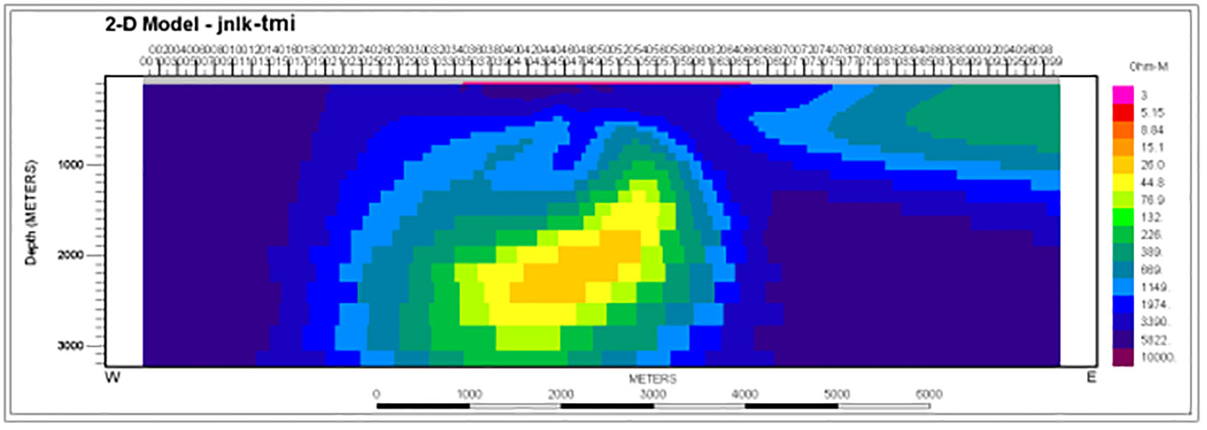
Figure 7: 2D inversion model of TM mode responses of all 26 MT sites along the Johnston Lake profile assuming a 2000 ohm-m background.
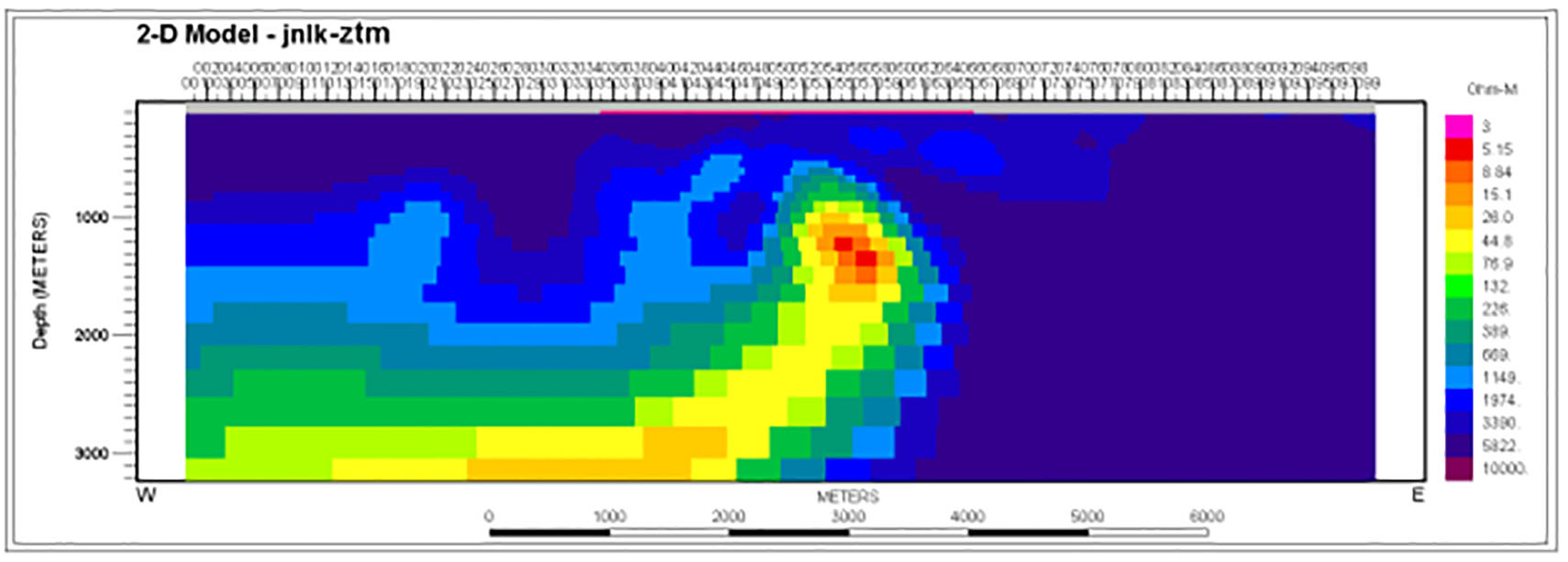
Figure 8: Joint inversion model of ZTEM and TM mode MT data.
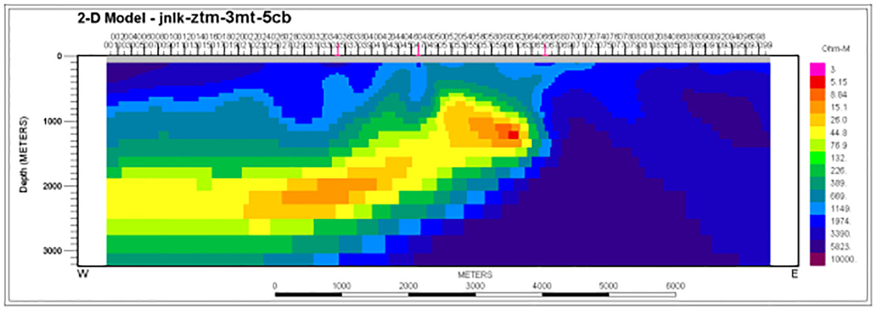
Figure 9: Joint inversion model of ZTEM & TM mode MT data from only three sites (red ticks).
Conclusion
The ZTMT2DIV algorithm is able to compute accurate resistivity inversion images over 2-D heterogeneity beneath topography through joint or separate inversion of ZTEM and ground MT data. Including MT, even a sparse number of sites appears to have good potential for improving the background resistivity and thus placing structure determined primarily by the ZTEM in its correct location. However, the limited number of tests here suggests that the MT sites should approximately span the length of the ZTEM profile to undergo joint inversion or else portions of the ZTEM model may become poorly constrained.
Acknowledgements
The authors wish to thank Geotech Ltd. for sponsoring this study. We gratefully thank Larry Petrie and Denison Mines Corp. for allowing use of the Johnston Lake ZTEM and Titan MT data.
<h4.References
De Lugao, P. P., and P. E. Wannamaker, 1996, Calculating the two-dimensional magnetotelluric Jacobian in finite elements using reciprocity: Geophysical Journal International, 127, 806–810.
Holtham, E., and D.W. Oldenburg, 2010, Three-dimensional inversion of MT and ZTEM data: 80th Meeting, SEG, Denver, Expanded Abstracts, 655-659.
Labson, V. F., A. Becker, H. F. Morrison, and U. Conti, 1985, Geophysical exploration with audio-frequency natural magnetic fields: Geophysics, 50, 656–664.
Legault, J.M., H. Kumar, B. Milicevic, and P. Wannamaker, 2009, ZTEM tipper AFMAG and 2D Inversion results over an unconformity uranium target in northern Saskatchewan, 79th Meeting, SEG, Houston, Expanded Abstracts, 1277-1281.
Lo, B., and M. Zang, 2008, Numerical modeling of ZTEM (airborne AFMAG) responses to guide exploration strategies: 78th Meeting, SEG, Las Vegas, Expanded Abstracts, 1098–1101.
Sasaki, Y, M.-J. Yi, and J. Choi, 2013, 3D inversion of ZTEM data for uranium exploration: 23RD International Geophysical Conference and Exhibition, ASEG, Extended Abstracts, 4p.
Spratt, J.E., C.G. Farquharson, and J.A. Craven, 2012. Analysis of magnetotelluric transfer functions to determine the usefulness of ZTEM data in the Nechako Basin, south-central British Columbia (parts of NTS 092O, N, 093B, C, F, G); in Geoscience BC Summary of Activities 2011, Geoscience BC Report 2012-1, 151–162.
Tarantola, A., 1987, Inverse problem theory, Elsevier, New York, 613 pp.
Wannamaker, P. E., J. A. Stodt, and L. Rijo, 1987, A stable finite element solution for two dimensional magnetotelluric modeling: Geophysical Journal of the Royal Astronomical Society, 88, 277-296.
Ward, S. H., 1959, AFMAG—Airborne and ground: Geophysics, 24, 761–787.