For a PDF of this paper click here.
PRESENTED AT SEG 2018
SUMMARY
We introduce an improved Airborne Inductively Induced Polarization (AIIP) mapping algorithm, which can extract with precision the three Cole-Cole parameters, i.e., low-frequency background apparent resistivity ρ0, Cole-Cole chargeability m and time-constant τ, while keeping the frequency factor c fixed. The derived Cole-Cole parameters (ρ0, m and τ) are related to physical properties. The interpretation of Cole-Cole parameters may be enhanced by considering the AIIP normalized chargeability m/ρ0 and the AIIP tau-scaled chargeability (TSC) m ⋅ τ. The former is analogous to the metal factor (MF). It responds well to most clays and is here given the label AIIP Clay Factor. The TSC is better suited for tracking relatively more chargeable materials with relatively longer Cole-Cole time-constants. The implications of AIIP normalized and tau-scaled chargeabilities for mineral exploration are demonstrated with cases from the Tli Kwi Cho kimberlite complex in Lac de Gras, NWT, Canada and the Cerro Quema high sulphidation epithermal gold deposits in Panama.
INTRODUCTION
Negative transients observed in helicopter TDEM data (Boyko et al., 2001) were attributed to Airborne Inductive Induced Polarization (AIIP) effects. In recent years, it has been widely accepted that the data acquired by helicopter TDEM systems reflect mainly two physical phenomena in the earth:
- Electromagnetic (EM) induction, related to the ground conductivity and governed by Faraday’s Law;
- Induced polarization (IP) effect related to the relaxation of polarized charges in the ground (Weidelt 1982 and Kratzer and Macnae 2012);
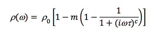
Pelton et al., 1978 were the first to demonstrate the suitability of the Cole-Cole impedance model to explain the results from IP/resistivity surveys and the amplitude and phase responses of various IP targets. Johnson (1984) applied the Cole-Cole model to time domain IP. Under the Cole-Cole model, the dispersive resistivity ρ(ω) is defined as,
 (1)
(1)
where ρ0 is the low frequency asymptotic resistivity, m (0≤m≤1.0) is the Cole-Cole chargeability in (V/V), τ is the Cole-Cole time-constant in seconds and ω=2πƒ, and c (0≤c≤1.0) is the frequency factor. The Cole-Cole time-constant is not the time-constant used to characterize a purely exponential decay, commonly used to model VTEM decays with no AIIP contribution. The four Cole-Cole parameters (ρ0, m, τ and c) are characteristic of the intrinsic polarizability of the ground. In general, the Cole-Cole chargeability m and time-constant τ depend on the quantity and size of polarizable material (Pelton et al., 1978). The frequency factor reflects the size distribution of the polarizable elements (Luo and Zhang, 1998).
An Improved AIIP Mapping Algorithm
The extraction of AIIP chargeability m using the Cole-Cole formulation from airborne TDEM data had been demonstrated by Kratzer and Macnae, 2012, Kwan et al., 2015, Viezzoli et al., 2017 and Kang et al., 2017.
The extraction of the four Cole-Cole parameters (ρ0, m, τ and c) from VTEM data can be challenging, due to the non-unique nature of the inverse problem. The original AIIP mapping algorithm introduced by Kwan et al., 2015 is computationally very slow and lacks precision. An improved version of AIIP mapping based on Airbeo from CSIRO/AMIRA[1] (Raiche 1998) applies the Nelder-Mead simplex minimization (Nelder and Mead, 1965) in the 2D (m,τ) plane. At each test point (mi, τi), the optimal low-frequency background resistivity ρ0 is found by one-dimensional Golden Section minimization (Press et al., 2002). The new AIIP mapping algorithm uses the Airbeo’s forward modeling kernel only. It can extract (ρ0, m, τ) parameters with precision while keeping c fixed at 0.7 for most cases.
AIIP tau-scaled chargeability m ⋅ τ and normalized chargeability m/ρ0
The Cole-Cole chargeability m is related to the quantity or volume percent/volume of chargeable material in the ground, and Cole-Cole time-constant τ is related to grain size; see Figure 1a taken from Pelton et al., 1978. The current range of AIIP tau sensitivity for VTEM systems operating with a base frequency of 25/30 Hz is 10-5 to 10-3 seconds. In the exploration for potentially economic sulphide mineralization, AIIP anomalies with relatively high sulphide content and fine-grained (in AIIP) are preferred as potential targets, as the region of interest highlighted by a red dashed ellipse.
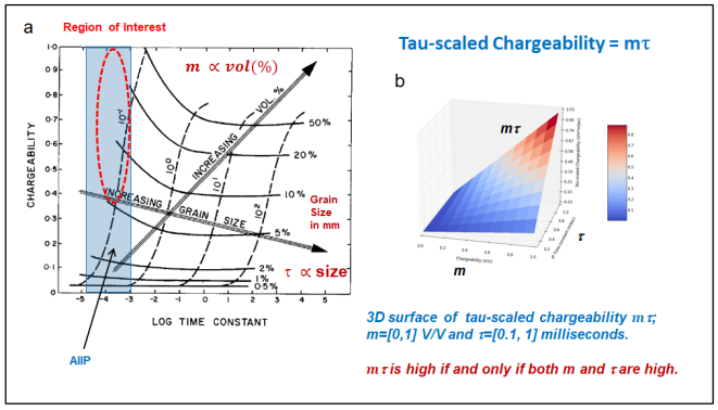
Figure 1: (a) Metallic sulphide content and grain size contours over the chargeability vs Cole-Cole time-constant (from Pelton et al., 1978), and (b) the m∙τ 3D surface plot showing high values occur only if both m and τ are high.
One way to select high chargeability m and high Cole-Cole time-constant τ anomalies is to use the product m ⋅ τ. As illustrated in Figure 1b, the surface m ⋅ τ is high if and only if both m and τ are high. The product m ⋅ τ can be considered as a good indicator of chargeable materials in the ground with relatively longer Cole-Cole time-constant or grain sizes in the order of 0.2 mm.
The ratio m/ρ0 was named by Lesmes and Frye, 2001, the normalized chargeability (MN), which was proposed first by Keller, 1959, and called the “specific capacity”. The normalized chargeability was further developed and interpreted by Slater and Lesmes, 2002. The normalized chargeability quantifies the magnitude of surface polarization and is proportional to quadrature conductivity. For non-metallic minerals, the quadrature conductivity is closely related to surface lithology and chemistry. Normalized chargeability varies linearly with clay content (Slater and Lesmes, 2002). Therefore, we called the normalized chargeability the AIIP Clay Factor (CF).
In frequency-domain galvanic IP the Metal Factor (MF) is defined as MF=2π×105FE/ρdc (Marshall and Madden, 1959), where FE=(ρdc-ρac)/ρac, and ρdc and ρac are apparent resistivities measured at DC and very high frequency (Slater and Lesmes, 2002). The frequency effect FE and the chargeability m are closely related (Slater and Lesmes, 2002, equations 11 and 12). Consequently, AIIP CF is analogous to MF in spectral IP for clays.
Tli Kwi Cho DO-27/DO18 kimberlites, Lac de Gras, NWT, CAN
The DO-27 and DO-18 are two well-known kimberlites in the Tli Kwi Cho (TKC) kimberlite complex, located about 360 kilometers NE of Yellowknife, Northwest Territories, Canada, in the Lac de Gras kimberlite cluster of the Archean Slave Craton, Jansen & Witherly, 2004 (Figure 2a). The kimberlites are located in the permafrost zone. The outline of the DO-27 and DO-18 is shown in Figure 2b. The magnetic signatures from the TKC kimberlites are easily identifiable (Figure 2c). DO-27 is coincident with a shallow-lake, while DO-18 is exposed (Figure 2d).
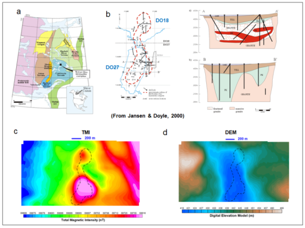
Figure 2: (a) The location of TKC complex in the Archean Slave Craton; (b) the outline of TKC complex and DO-27/DO-18 kimberlites, and two geological sections over DO-27 (from Jansen & Doyle, 2000); (c) and (d) The total magnetic intensity and digital elevation data acquired from the helicopter VTEM survey.
The improved AIIP mapping is applied to the helicopter VTEM data over the two pipes. The Z-component dB/dt voltage data in off-time windows from 0.12 milliseconds to 6.9 milliseconds are used. Cole-Cole parameters (ρ0, m, τ) are derived using a fixed frequency factor c of 0.7.
The AIIP CF data in (mV/V*S/m) and TSC data in (V/V*Milliseconds) are shown side by side in Figure 3. They look quite similar (Figure 3c). The distribution pattern of both seems to be spatially associated with the TKC kimberlite complex, and they almost match perfectly with DO-27, strongly suggesting that the AIIP effects over the TKC kimberlites are related to clay. However, the electrical properties of DO-18 and DO-27 are different, as the former is quite resistive and the latter relatively conductive (Figure 3b). Kang et al. 2017 suggest that the AIIP source may be a frozen ice/clay mixture (highly resistive) at DO-18 and conductive clay for DO-27 and both show strong chargeable responses (Figure 3a). We agree. In the study of Drybones Bay kimberlite, NWT, Kaminsky & Viezzoli, 2017 concluded also that the clay in the lake sediments is the main source of AIIP effects.
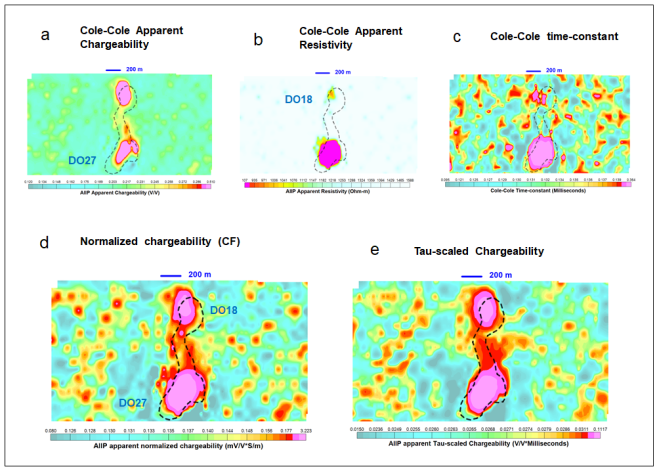
Figure 3: Cole-Cole (a) apparent chargeability, (b) apparent resistivity, (c) time-constant, (d) The normalized chargeability or Clay Factor (CF), and (e) the TSC over the TKC complex;
It is worth noting that the CF and TSC data being quite similar over the TKC complex. For non-metallic minerals at low frequencies (f≤1000 kHz), the imaginary part of the low-frequency complex conductivity can be considered a function of the surface conductivity, and the imaginary component is primarily indicative of the surface polarization, Slater & Lesmes, 2002. The Cole-Cole time-constant τ is proportional to the surface area of clay grains, i.e., τ≈kr2, where k is a constant and r is the radius of the chargeable grain (Revil, Florsch & Mao, 2015), or TSC=mτ≈mkr2. CF and TSC are related to the surface conductivity/polarization and specific surface area of clay, and hence their similarities.
Cerro Quema high sulphidation epithermal gold deposits, Panama
A helicopter-borne VTEM, magnetic and gamma-ray spectrometric survey was carried out in March 2012 over the Cerro Quema high sulphidation epithermal gold deposits located in the Azuero Peninsula, Panama, Figure 4a. The survey was flown on behalf of Pershimco Resources Inc.
The study area consist of mainly sedimentary, volcaniclastic and extrusive volcanic rocks of the Rio Quema Formation, deposited in a forearc basin, overlying the Azuero Igneous Basement, Corral et al. 2011, Figure 4d. The Cerro Quema gold deposits (La Pava, Quemita and Quema) are hosted in the Upper Unit of the Rio Quema Formation, an east to west trending belt of porphyritic, pyroclastic flows, and lavas of dacite and andesite composition. The Rio Joaquin Fault is located to the south of the deposits. The deposits are located in elevated grounds, Figure 4b.
Three alteration types are identified by detailed geologic mapping and drill core logging: silica-pyrite, clay-pyrite and propylitic alteration (Valliant et al., 2011), Figure 4c.
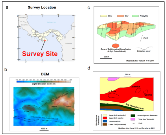
Figure 4: (a) Survey area; (b) The Digital Elevation Model (DEM) data; (c) Alterations section over the La Pava deposit (after Valliant et al., 2011); (d) General geology of the study area (after Corral et al., 2011).
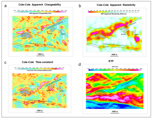
Figure 5: Cole-Cole (a) apparent chargeability, (b) apparent resistivity, (c) time-constant and (d) RTP data from Cerro Quema.
AIIP mapping of Cerro Quema helicopter TDEM data was carried out using c=0.7. The AIIP apparent chargeability data are shown in Figure 5a. The strong chargeable responses are located around La Pava and along the interpreted contact north of the deposits. The AIIP apparent resistivity data are shown in Figure 5b. Two conductive trends can be seen, the contact trend and the Quemita-Quema trend. The Cole-Cole time-constant data are shown in Figure 5c, with higher values located around La Pava, the contact and the Rio Joaquin Fault. The RTP data are displayed in Figure 5d, showing clear association of the magnetic data with the inferred contact and the Rio Joaquin Fault.
The AIIP CF data are shown in Figure 6a, side by side with the TSC data in Figure 6b. The CF data maps the clay alterations. In Cerro Quema, we see clear separation between the CF and the TSC. Most of the CF highs are located in the low lying areas north of the interpreted contact, south of the Rio Joaquin Fault, and the southern base of the mountain hosting the Quemita and Quema deposits. Most of the TSC highs are located along the interpreted contacts north of the Cerro Quema deposits, along the Rio Joaquin Fault and in the halos surrounding the La Pava and south of the Quemita. In this case study, the TSC data better reflects the disseminated and fine-grained pyrite alteration halos. The semi-circular halos could potentially be used an exploration vectors for high sulphidation epithermal gold mineralization.
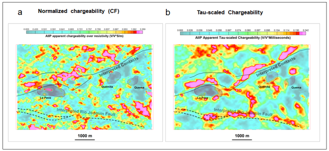
Figure 6: A clear divergence is seen between (a) the CF data and (b) the TSC data from Cerro Quema.
DISCUSSIONS
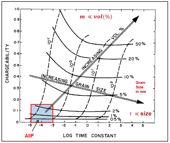
Figure 7: AIIP zone of interest for low concentrations of disseminated metallic sulphides in a resistive host; chargeability vs. time constant plot from Pelton et al., 1978.
Many Canadian Archean lode gold deposits in glaciated terrains are chargeability and resistivity highs. Therefore the mρ0 and ρ0 maps could potentially be used for targeting these kinds of mineralization.
Many Archean lode gold deposits and most disseminated sulphide ores are considered ‘fine-grained’ in ground IP, in contrast to coarse grained stringer to massive sulphides. They show high resistivities and short time constants.
For potential Archean lode gold mineralization with low sulphide concentration, low chargeability and variable Cole-Cole time-constant, as illustrated in Figure 7, the τρ0 and ρ0 maps could be potential targeting tools as well.
The AIIP resistivity and resistivity-associated maps should be interpreted in conjunction with magnetic maps, since many explorationists look for lode gold in areas of magnetite depletion, due to hydrothermal alteration.
CONCLUSIONS
We have developed an improved AIIP mapping algorithm to extract Cole-Cole parameters from helicopter TDEM (VTEM) data. The method has been proven to be efficient and robust, and is capable of obtaining precise Cole-Cole parameters (ρ0, m, τ) while keeping c fixed.
We have found that the interpretation of the derived Cole-Cole parameters can be enhanced by the use of AIIP normalized chargeability (m/ρ0) and AIIP tau-scaled chargeability (TSC) m ⋅ τ . The former can be treated as an indicator of very fine-grained polarizable materials, such as clay, and is named the AIIP Clay Factor (CF). The AIIP TSC is considered to be a good indicator of relatively more chargeable fine-grained materials with relatively longer Cole-Cole time-constants or grain sizes in the range of 0.2 mm.
AIIP mapping results from TKC kimberlite complexes in NWT Canada and Cerro Quema high sulphidation epithermal gold deposits in Panama indicated the AIIP CF and TSC can be used to separate clay-dominated and fine-grained disseminated metallic sulphide-dominated polarizable materials in the ground.
ACKNOWLEDGEMENTS
The AIIP mapping algorithm is based on Airbeo from project P223F CSIRO/AMIRA.
We would like to thank University of British Columbia for providing the helicopter VTEM data over the TKC kimberlite complex, Lac de Gras, NWT, and Pershimco Resources Inc. for permission to use the airborne geophysical survey data over the Cerro Quema gold deposits, Panama. Finally, Geotech is thanked for permission to publish the AIIP mapping results.
REFERENCES
Boyko, W., N.R. Paterson, and K. Kwan, 2001, AeroTEM characteristic and field results: The Leading Edge, 20, 1130–1138, https://doi.org/10.1190/1.1487244.
Cole, K., and R. Cole, 1941, Dispersion and absorption in dielectrics, Part I. Alternating current characteristics: Journal of Chemical Physics, 9, 341–351, https://doi.org/10.1063/1.1750906.
Corral, I., A. Griera, D. Gómez-Gras, M. Corbella, À. Canals, M. Pineda-Falconett, and E. Cardellach, 2011, Geology of the Cerro Quema Au-Cu deposit: Geologica Acta, 9, 481–498, https://doi.org/10.1344/105.000001742.
Jansen, J., and K. Witherly, 2004, The Tli Kwi Cho kimberlite complex, Northwest Territories, Canada: A geophysical case study: 74th Annual International Meeting, SEG, Expanded Abstracts, 1147–1150, https://doi.org/10.1190/1.1839654.
Jansen, J. C., and B. J. Doyle, 2000, The Tli Kwi Cho Kimberlite Complex, Northwest Territories: A Geophysical Post Mortum. Johnson, I. M., 1984, Spectral induced polarization parameters as determined through time-domain measurements: Geophysics, 49, 1993–2003, https://doi.org/10.1190/1.1441610.
Kaminski, V., and A. Viezzoli, 2017, Modeling induced polarization effects in helicopter time-domain electromagnetic data: Field case studies: Geophysics, 82, no. 2, B49–B61, https://doi.org/10.1190/geo2016-0103.1.
Kang, S., D. Fournier, and D. W. Oldenburg, 2017, Inversion of airborne geophysics over the DO-27/DO-18 kimberlites – Part 3: Induced Polarization: Interpretation, 5, no. 3, T345–T358, https://doi.org/10.1190/int-2016-0141.1.
Keller, G. V., 1959, Analysis of some electrical transient measurements on igneous, sedimentary and metamorphic rocks, in WaitJ. R., ed., Overvoltage research and geophysical applications: Pergamon Press, 92–111.
Kratzer, T., and J.C. Macnae, 2012, Induced polarization in airborne EM: Geophysics, 77, no.5, E317–327, https://doi.org/10.1190/geo2011-0492.1.
Kwan, K., A. Prikhodko, J. M. Legault, G. Plastow, J. Xie, and K. Fisk, 2015, Airborne inductive induced polarization chargeability mapping of VTEM data, Expanded Abstract, ASEG-PESA 2015.
Lesmes, D. P., and K. Frye, 2001, Influence of pore fluid chemistry on the complex conductivity and induced polarization responses of Berea sandstone: Journal of Geophysical Research, 106, 4079–4090, https://doi.org/10.1029/2000jb900392.
Luo, Y., and G. Zhang, 1998, Theory and application of Spectral Induced Polarization, Geophysical Monograph Series. Marshall, D. J., and T. R. Madden, 1959, Induced polarization, a study of its causes: Geophysics, 24, 790–816, https://doi.org/10.1190/1.1438659.
Nelder, J. A., and R. Mead, 1965, A simplex method for function minimization: Computer Journal, 7, 308–313, https://doi.org/10.1093/comjnl/7.4.308.
Pelton, W. H., S. H. Ward, P. G. Hallof, W. R. Sill, and P. H. Nelson, 1978, Mineral discrimination and removal of inductive coupling with multifrequency IP: Geophysics, 43, 588–609, https://doi.org/10.1190/1.1440839.
Press,W. H.,S.A. Teukolsky, W. T. Vetterline, andB. P. Flannery, 2002, Numerical recipes in C: The art of scientific computing, 2nded., Cambridge University Press.
Raiche, A., 1998, Modelling the time-domain response of AEM systems: Exploration Geophysics, 29, 103–106, https://doi.org/10.1071/eg998103.
Revil, A., N. Florsch, and D. Mao, 2015, Induced polarization response of porous media with metallic particles– Part 1: A theory for disseminated semiconductors: Geophysics, 80, no. 5, E525–D538, https://doi.org/10.1190/geo2014-0577.1.
Slater, L. D., and D. P. Lesmes, 2002, IP interpretation in environmental investigations: Geophysics, 67, 77 –88, https://doi.org/10.1190/1.1451353.
Valliant, W. W., S.E. Collins, and H. Krutzelmann, 2011, Technical Report on The Cerro Quema Project, Panama, NI43-101, prepared for Pershimco Resources Inc., by Scott Wilson Roscoe Postle Associates Inc.
Viezzoli, A., V. Kaminski, and G. Fiandaca, 2017, Modeling induced polarization effects in helicopter time domain electromagnetic data: Synthetic case studies: Geophysics, 82, no. 2, E31–E50, https://doi.org/10.1190/geo2016-0096.1.
Weidelt ,P., 1982, Response characteristics of coincident loop transient electromagnetic systems: Geophysics, 47, 1325–1330, https://doi.org/10.1190/1.1441393.
Witherly, K., R. Irvine, and E. B. Morrison, 2004, The Geotech VTEM time domain electromagnetic system: 74th Annual International Meeting, SEG, Expanded Abstracts, 1217–1221, https://doi.org/10.1190/1.1843295..
[1] Commonwealth Scientific and Industrial Research Organization and Amira International;