For a PDF of this paper click here.
PRESENTED AT AEM 2018
SUMMARY
We present the results of advanced processing and Spatially-Constrained Inversions (SCI) applied to TDEM data obtained from a helicopter-borne EM survey conducted over the Wahpeton aquifer, located in North Dakota.
The obtained 1D resistivity model helped map and differentiate the sedimentary layers that overlie a more resistive Precambrian granitic basement. The main aquifer that is associated with glacial drifts and composed of sand and gravel is accurately imaged. This unit is located at shallow depth and occurs as interbedded between two clay units. The comparison of the inversion outcomes with available borehole results has shown a good agreement in layer thickness estimates.
The integration of the 3D image of the aquifer obtained with advanced processing and inversion techniques of the EM data with available borehole data will support better management of water resources within this area.
Key words: AEM, Wahpeton, Aquifer, 1D inversion, Spatially-Constrained Inversion (SCI).
INTRODUCTION
Buried valley aquifers, consisting of permeable sand and gravel deposits in glacial and bedrock valleys, are important sources of groundwater supply in many regions of the United States and Canada. These aquifers have been difficult to define because they are often partially eroded, have complex lithology, and are hidden by other shallow sand and gravel aquifers within thick glacial overburden.
Investigations of the Spiritwood glacial aquifer near Jamestown, North Dakota, in October 2016, by the North Dakota State Water Commission (NDSWC) showed that airborne time domain electromagnetic (TDEM) surveys helped aquifer mapping and characterization (Legault et al., 2017).
Following the success of the Spiritwood JT survey, the NDSWC commissioned another helicopter-borne EM survey over the near Wahpeton, ND in Fall 2017. The Wahpeton survey bock consisted of nearly 2000 line-km of coverage along a roughly 10-20 km wide by 100 km long north-south corridor over the Wahpeton Aquifer System, lying just west of the Red River and the Minnesota State border, and roughly extending from the city of Fargo in the north, to Wahpeton in the south.
The EM data collected over the Wahpeton Aquifer System have been inverted with a layered-earth algorithm to produce resistivity-depth models. These models resolve the location and depths to the top and bottom of the aquifer, thus providing a detailed picture of the aquifer geometry and the associated stratigraphic units. Advanced processing and inversion complemented with integration of existing data (i.e. well data, hydrogeological data) allowed a superior image of the aquifers in three dimensions providing the State with an enhanced framework for their groundwater management.
METHOD AND RESULTS
Helicopter-borne EM survey
The Project area lies within the Wahpeton and Fargo areas of North Dakota. The helicopter-borne EM survey was flown in November 2017. Initially, a reconnaissance survey was flown at large line spacing of 5 km. Based on preliminary EM data inversion results infill-lines, spaced at 500m apart were flown to provide higher detail in the results. In total, 2014 line-km were flown along EW oriented traverses. Tie lines were flown in the NS direction and were spaced at 5 km apart (Figure 1).
The average EM system ground clearance was 35m. The maximum flight heights were encountered over cultural features such as large power lines. Additionally to the EM data acquisition, the VTEM system collected Total Field magnetic data. The magnetic field signal is useful for determining deep seated geological contacts and is also valuable for locating intrusive bodies. Since neither of those was the target of the survey within the NDSWC Wahpeton survey area and therefore, the magnetic interpretation is not considered here. A power line monitor was used to collect 60 Hz industrial noise. The acquired EM data were calibrated using borehole logs from two test holes downloaded from the website http://mapservice.swc.nd.gov.
The acquired test data are calibrated with an amplitude scale factor based on forward and inversion results obtained from the test holes.
Inversion procedure
The collected EM data were processed and inverted using the Laterally Constrained Inversion (LCI) algorithm of Aarhus Workbench v.5.5.00 (Aarhus Geosoftware, 2017). The data contaminated with power line noise were removed prior to inversion. Two-step processing stages were applied to the data: automatic and manual processing. During the automatic processing, DGPS data were filtered using a step-wise polynomial filter and the altitudes were corrected using a series of polynomial filters. Next, the data were filtered using a trapezoidal spatial averaging filter. Manual filtering consisted mainly in EM coupling removal so that data affected by power line noise were removed. Data collected at heights greater than approximately 60 m above the ground surface were also removed due to low signal level. Given its superior accuracy compared to the acquired Digital Elevation Model (DEM), the National Elevation Model (NED) was used as a reference for all elevations. The 1arc-second resolution NED dataset was downloaded from the National Map Website (U.S. Geological Survey, 2016).
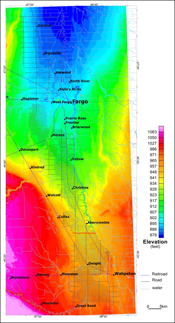
Figure 1: Flight path over the 1 arc-second NED image. The red line is the trace of line L1424, whose field and inversion results are shown in Figure 3.
After the data have been processed, they were inverted using an LCI (Christensen at al., 2007), which uses nearby soundings along the flight lines as constraints. The profile and depth slices were examined, and any remaining electromagnetic couplings were masked out of the dataset. LCI vertical constraints on the resistivity were set at 2.7 and at 1.6 for the horizontal resistivity constraints with a reference distance of 100 m. A 30-layer smooth model was used in the LCI. The thickness of the first layer was set to 3 m, and the thickness of subsequent layers was expanded by a factor of 1.08, to reach a maximum thickness of 25m for the last layer.
Further to LCI inversions, Spatially-Constrained Inversions (SCI) were performed on the processed dataset. Unlike the LCI, which uses only the data acquired along flight lines, the SCI makes use of data along and across flights lines within user-specified distance criteria (Viezzoli et al., 2008). The spatial reference distance was set to 75 m and the vertical and lateral constraints were set to 2.4 and 1.3 respectively for all layers. These parameters provided both a reasonable and constrained, yet smooth, result.
Since the sensitivity of any AEM system decreases with depth, a 5-layer model study was performed to determine the ability to recover deep-seated resistivity structures . The study model includes two layers, each 30 m thick and 50 Ohm-m in resistivity, hosted by 10 ohm-m host rock. The top of the 1st layer is located at depth of 10m and the top of the second layer, at 60m. Figure 2 presents the sensitivity of the system and the inversion to recover the initial model (red curve). The blue curve, which represents the inverted results, shows that the recovered resistivity for the shallower layer is around 40 ohm-m, whereas it is 20 ohm-m for the deeper one. In other words, the sallower layer is better resolved than the deeper one due to decrease of the system sensitivity with depth.
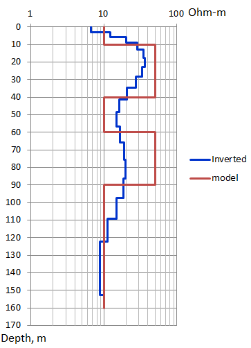
Figure 2: Model study used for sensitivity analysis.
Hydrogeological context
The survey area lies within the Red River Valley, a flat and gently dipping plain formed as the result of silt and clay sediments on the floor of former glacial Lake Agassiz (Schafer and Sagsveen, 1999).
Surface water is a vital resource to North Dakota cities, industry and agriculture. The Missouri River discharge is the largest quantity and the best quality of all rivers in North Dakota. Ground water resources occur in two principal aquifer types: (1) unconsolidated glacial deposits, and (2) sedimentary bedrock. Within the survey area, the majority of high quality water is contained in glacial drift aquifers that are generally composed of sand and/or gravel deposited by glacial activity. Most of them are located at or near the surface. However, some of them are deeply buried by till deposits (Schafer and Sagsveen, 1999).
The surface geology of the survey area consists mainly of a Quaternary system (Holocene and Pleistocene) that is composed of glaciolacustrine interbedded sands, silts, gravels, clays and silty clays (Anderson, 2005). The sedimentary formations are overlying a granitic Precambrian basement. The thickness of the sediments is variable up to 600 feet (Bluemle, 2003).
Inversion results
Figure 3 shows the SCI results for line L1424 located in the southern portion of the survey area at 3.5 km south of Abercrombie and 20 km, approximately northwest of Wahpeton. The top panel presents the gated raw data and the middle panel presents the 60 Hz power line noise monitoring channel; the peaks indicate higher noise levels. The bottom panel of Figure 3 is the 1D-resistivity section extending from the surface (elevation ≈ 950 feet) to an elevation of about 200 feet. The white zones in the sections are areas not inverted due to the power line effects. The granitic basement, highlighted by elevated resistivity values > 150 ohm-m, occurs at depths ranging from 350 feet to 450 feet approximately. It appears to be gently dipping westward. The overlying sediments are characterized by lower resistivity values ranging from <10 ohm-m to up to approximately 100 ohm-m. The sedimentary package consists mainly of three layers with various thicknesses and electrical properties, which are from top to bottom: (1) upper clay unit [5-10] ohm-m with an average thickness of 60 feet; (2) banded sand unit [30-100] ohm-m with an average thickness of 180 feet; and (3) lower clay unit [5-20] ohm-m with an average thickness of 200 feet. The banded sand formations are considered to be the main lithological unit that hosts water resources.
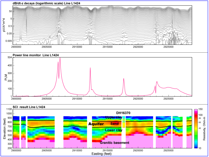
Figure 3: SCI result for line L1424, whose trace is highlighted in Figure 1. From top to bottom, VTEM decays in logarithmic scale, Power line monitor and 1D resistivity section obtained with SCI. The white areas in the section were not inverted due to power line noise. The inferred top and bottom of the aquifer are shown in black. The litho-stratigraphic column shown between eastings of 2915000 and 292000 is obtained from well DH16370.
To assess the inversion accuracy the lithology log obtained from borehole DH16370 is plotted in the resistivity section. As shown in Figure 3, the borehole results are in good agreement with the SCI results.
Figure 4 shows 1D resistivity depth slices corresponding to various depth levels and Figure 5 presents a perspective view of 3D-resistivity voxel obtained from the SCI results. The yellow feature, which corresponds to a resistivity range defined by lower and upper boundaries of 36 and 110 ohm-m, respectively, is suggested to be attributed to banded sand formations and the pink zone corresponding to resistivity values > 110 ohm-m is attributed to the granitic basement.
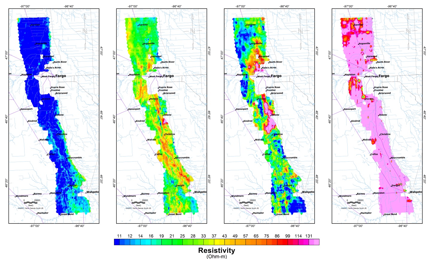
Figure 4: Resistivity depth slices corresponding to depth levels: a) 32-44 feet, b) 143-146 feet, c) 267-298 feet and d) 599-665 feet.
![Figure 5: 3D voxel obtained from SCI inversion of VTEM data. The pink colour represents the resistivity range >110 ohm-m (corresponding to granitic basement) and the yellowish zone corresponds to the resistivity range [36-110] ohm-m over a depth range of [0-300] feet. The top layer with higher tranparency represents the surface. Vertical exaggeration=×10. The view is looking to the NE. Coordinates are in feet.](https://www.geotech.ca/wp-content/uploads/2018/12/wahpeton-figure-5.png)
Figure 5: 3D voxel obtained from SCI inversion of VTEM data. The pink colour represents the resistivity range >110 ohm-m (corresponding to granitic basement) and the yellowish zone corresponds to the resistivity range [36-110] ohm-m over a depth range of [0-300] feet. The top layer with higher tranparency represents the surface. Vertical exaggeration=×10. The view is looking to the NE. Coordinates are in feet.
CONCLUSIONS
The helicopter-borne EM data acquired over the Wahpeton Aquifer System have been processed and inverted with Spatially-Constrained Inversion algorithm to image the subsurface geology. The inversion outcomes provide a good image and more detailed characterization of the aquifer geometry and the stratigraphic units. Advanced processing and inversion complemented with integration of existing well data and hydrogeological information allowed a superior image of the aquifer in 3D providing an enhanced framework for groundwater management.
ACKNOWLEDGMENTS
We are grateful to North Dakota State Water Commission for permission to publish these results.
REFERENCES
Aarhus Geosoftware, 2017 Aarhus Workbench: https://www.aarhusgeosoftware.dk/aarhus-workbench (Accessed January 24, 2018)
Bluemle, J.P., 2003, Generalized Bedrock Map of North Dakota, North Dakota Geological Survey, North Dakota Miscellaneous Maps, MM-36 https://www.dmr.nd.gov/ndgs/Publication_List/ndmisc.asp (Accessed Jan 22, 2018).
Christensen, N. B., Reid, J. E., and Halkjaer, M., 2009, Fast, laterally smooth inversion of airborne time-domain elecromagnetic data. Near Surface Geophysics 599-612.
Legault, J.M., Eadie, T., Plastwow, G., and Prikhodko, A., 2017, Spiritwood valley aquifer characterization using helicopter TDEM system, SAGGEP-NGWA 2017- Denver, Colorado.
Schafer, E.T., and Sagsveen, M.G., 1999, North Dakota, Source Water Assessment Program, Divion of Water Quality.
U.S. Geological Survey (USGS), 2016, The National Map, 2016, 3DEP products and services: The National Map, 3D Elevation Program Web page, http://nationalmap.gov/3DEP/3dep_prodserv.html (Accessed January 24, 2018).
Viezzoli, A., Christiansen, A. V. , Auken, E., and Sorensen, K., 2008, Quasi-3D modeling of airborne TEM data by spatially constrainted inversion. Geophysics, 73 (3), F105-F11.